Linear algebra studies vectors, linear combinations, linear maps and systems of linear equations. In quantitative finance, it gives a common language for turning positions into exposures, matching cash flows and organising return data. Its central operation is simple: multiply building blocks by quantities, then add them.
A vector keeps quantities in a fixed order; a matrix records how those quantities contribute to several outputs. The ordering and units are part of the model, even though the arithmetic cannot check them for you.
From three assets to two exposures
Consider a synthetic one-period return-factor model. Portfolio weights are fractions of starting portfolio value, in asset order A, B, C. Rows of the loading matrix correspond to factors F1, F2; columns retain the same asset order:
Both asset returns and factor returns are expressed as decimal fractions over the same period, so these loadings are dimensionless. With fixed loadings, matrix multiplication gives the portfolio's factor exposure:
Each row takes a dot product with the weights. Equivalently, the result is a linear combination of the matrix columns: 40% of A's loading vector, plus 30% of B's, plus 30% of C's.
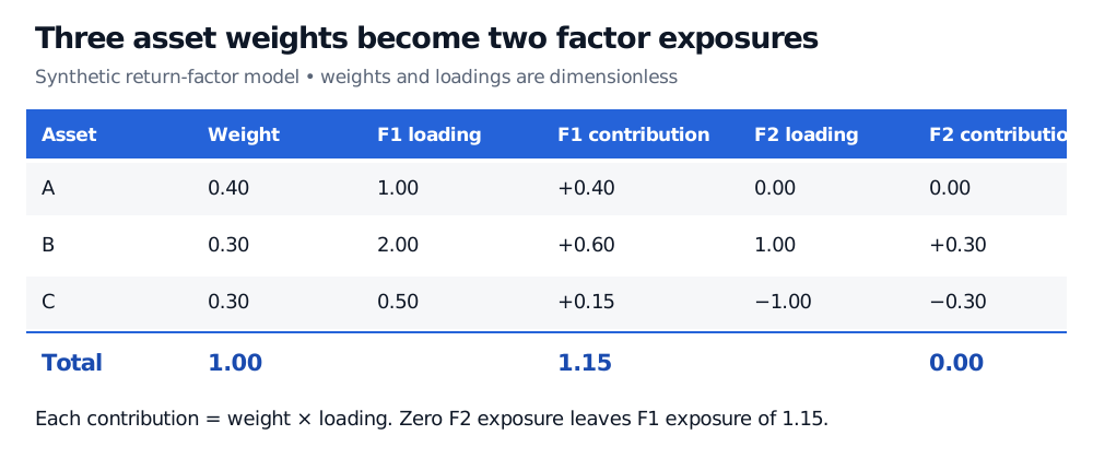
Original synthetic return-factor example. Contributions are weight times dimensionless loading; asset and factor orders remain fixed.
For interpretation, suppose the model is , where is an asset-specific residual return. Then, for beginning-of-period weights and no interim trading, external cash flows or costs,
If F1 returns 1%, F2 returns 2% and all residuals are zero, portfolio return is 1.15%. The exposure 1.15 alone is not a return forecast. Zero F2 exposure means neutrality to that factor within this fixed linear model; F1 exposure, residual risk and model error remain.
Calculating a result versus finding the weights
A linear map preserves addition and scaling:
This lets desks aggregate books before or after computing exposures. Doubling every position doubles the mapped exposure. A fully invested weight vector must also satisfy ; doubling these weights describes exposure relative to the original capital base and requires a separate financing convention.
Run the question backwards and you obtain a system of linear equations: choose so that for a target exposure . The columns' span determines which targets are attainable. The rank and null space determine whether different holdings can produce the same target. Budget limits, short-sale restrictions and transaction costs add further requirements; matching measured exposures alone does not establish an affordable hedge.
Other branches answer different practical questions. Least squares fits an approximate match when an exact system is inconsistent. A basis provides independent coordinates. Eigenvalues and eigenvectors help identify directions of variation in covariance analysis.
Using linear algebra does not make every calculation linear
Portfolio variance uses the covariance matrix through the quadratic form
For fixed , doubling the exposure vector multiplies variance by four, rather than two. A genuine covariance matrix is positive semidefinite, which ensures nonnegative variance. Nonlinear payoffs and changing factor loadings also require more than a fixed exposure map.
To practise the arithmetic, read Vectors and Matrices. For the column-space interpretation, replication systems and covariance-ready matrices, continue with Vectors, Matrices and Linear Systems, part of the Linear Algebra, Optimisation and Numerical Methods Programme. Both have public previews; full lessons require membership.
Sources
- Gilbert Strang, Introduction to Linear Algebra, 5th edition, Wellesley–Cambridge Press, 2016, §1.3 (matrix–vector products and linear equations) and Chapter 3 (vector spaces and subspaces).
- MIT OpenCourseWare, The Geometry of Linear Equations, 18.06SC, Fall 2011 — row, column and matrix views of linear systems.