Matrix multiplication forms row-column sums and composes linear maps. Follow strategy quantities through asset holdings into factor sensitivities, and distinguish regrouping, reordering and entrywise products.
Matrix multiplication
Matrix multiplication combines two matrices by taking a row from the first and a column from the second, multiplying their corresponding entries, and summing. Its central use is to combine successive linear transformations: one matrix turns strategy quantities into asset positions; another turns those positions into factor sensitivities. Their product maps strategies straight to sensitivities.
The shared dimension is the handoff
For A with m rows and n columns, and B with n rows and p columns,
m×nAn×pB=m×pC,cij=k=1∑naikbkj.
The inner dimensions must agree: each row of A and each column of B must contain the same number of entries. The result keeps the outer dimensions. Entry cij is the dot product of row i of A with column j of B.
There is a second reading: column j of AB is A applied to column j of B. Each column of B describes one input recipe; the corresponding column of AB gives that recipe's final output. These are two views of the same calculation. MIT's lecture notes develop these row and column views alongside other ways of forming a product.
A shape check is necessary; names and units must agree too. If A's columns refer to assets in a particular order, B's rows must use that same order. Matching three columns with three rows cannot detect a swapped asset label.
A two-stage risk calculation
Consider a hypothetical desk with two strategies and three assets. One unit of strategy 1 holds one lot each of assets 1 and 3. One unit of strategy 2 holds one lot each of assets 2 and 3. The bundle matrix is
B=101011.
Rows identify assets; columns identify strategies. Entry bij measures asset-i lots per unit of strategy j. For strategy quantities x=(2,3)T, the holdings vector is
Bx=235.
Now specify two risk factors. Each factor move is measured in basis points, and each asset has the following fixed local P&L sensitivities:
A=[102101].
Rows identify factors; columns identify the same three assets. Each entry measures USD per basis point per asset lot. For example, one lot of asset 2 contributes USD 2 per bp to factor 1 and USD 1 per bp to factor 2. The two portfolio sensitivities are
A(Bx)=[1(2)+2(3)+0(5)0(2)+1(3)+1(5)]=[88]USD per bp.
These are separate sensitivities to the specified factors, rather than two cash payments. Under this local model, a one-bp move in factor 1 with factor 2 unchanged gives approximately USD 8 of P&L. Changing both factors requires their respective moves. Larger moves can require nonlinear repricing; multiplying sensitivities does not establish exact payoff replication or remove unmeasured risks.
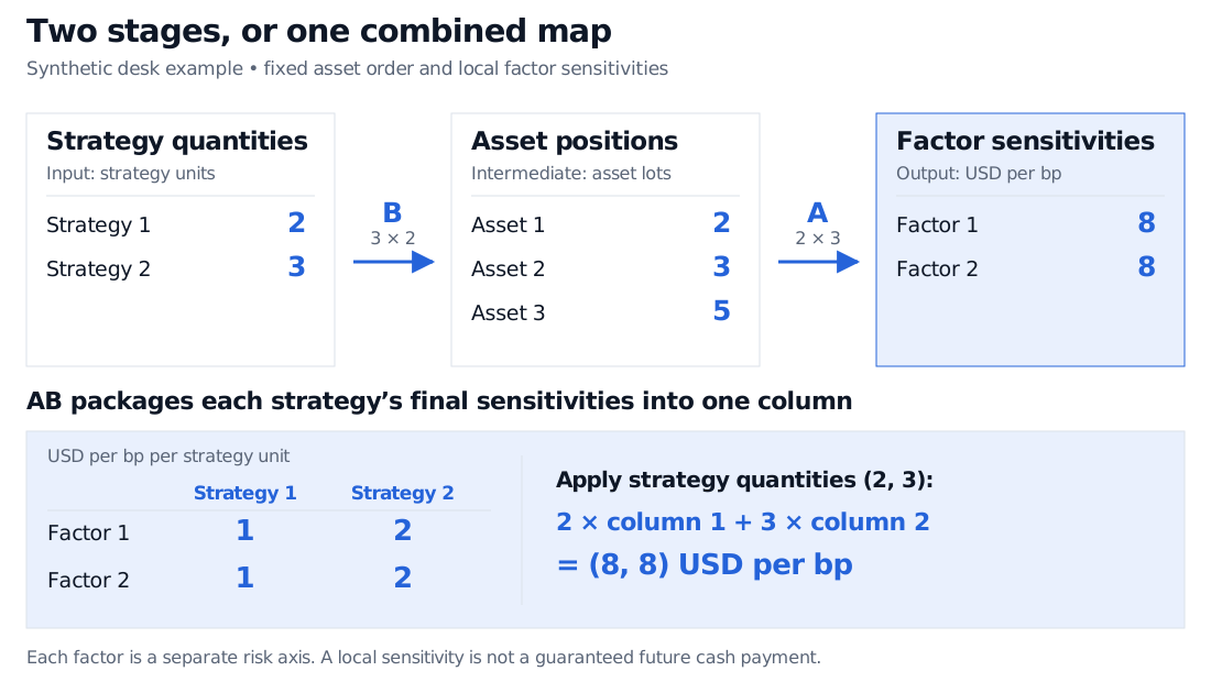
Two strategy quantities, 2 and 3, map through B into asset lots 2, 3 and 5, then through A into two sensitivities of USD 8 per bp. The shortcut AB has columns 1,1 and 2,2, measured in USD per bp per strategy unit.
Original synthetic example. The intermediate three-asset book and the combined two-strategy map produce the same two factor sensitivities. All asset and factor orders are fixed.
The first column is strategy 1's two sensitivities; the second is strategy 2's. Their units are USD per bp per strategy unit. Thus
(AB)x=[1(2)+2(3)1(2)+2(3)]=[88]=A(Bx).
A desk evaluating many strategy allocations can reuse AB while the bundle definitions and sensitivities stay fixed. If either changes, the combined map must change as well. For a single calculation, keeping the two matrix-vector steps may avoid forming a larger product unnecessarily.
Regrouping preserves order; reordering changes the map
Matrix multiplication is associative: for compatible matrices, (AB)C=A(BC). Parentheses select which intermediate result to calculate first; the matrices retain their order. With column vectors, ABx applies B first and then A.
It is generally not commutative. AB and BA may have different shapes, one may be undefined, and even same-size square matrices need not give equal products. Here both numerical products exist, but
AB=[1122]is 2×2,BA=101213011is 3×3.
Algebraic compatibility does not create an economic reverse workflow. In the desk example, A outputs factor sensitivities, whereas B expects strategy quantities. The two-dimensional arrays fit numerically, but their labels and units do not describe the same interface. Treating BA as a meaningful financial operation would require a separately defined interpretation. It is also not an inverse of AB.
The same discipline matters for a covariance matrix: the asset order in every adjacent vector or matrix must match. Correct dimensions alone do not establish a correct risk calculation.
Multiplying corresponding entries is a different operation
The Hadamard product, written A∘D, multiplies entries in the same positions: (A∘D)ij=aijdij. It requires equal shapes and preserves that shape. It does not perform the row-column sums that compose two maps.
For the combined map C=AB above and the 2×2 identity matrix I2,
CI2=C=[1122],C∘I2=[1002].
Ordinary multiplication by the identity preserves the map. Entrywise multiplication by the identity masks its off-diagonal entries. Both operations are useful, but answer different questions.
For a fuller treatment, Matrix Algebra: Operations, Rules, and the Transpose develops product laws and transpose identities (membership for the full lesson; public preview). Vectors and Matrices introduces matrix-vector products through portfolio factor exposures with the same access arrangement.
Sources
Gilbert Strang, Introduction to Linear Algebra, 5th edition, Wellesley–Cambridge Press, 2016, §2.4, “Rules for Matrix Operations,” pp. 70–73. Dimensions, row-column products, associativity and order.