Dot product: Definition & Examples

The dot product multiplies matching entries of two real vectors, then adds the products. It returns one number, a scalar:

\mathbf{x}\cdot\mathbf{y} =\mathbf{x}^{\mathsf T}\mathbf{y} =\sum_{i=1}^{n}x_i y_i.

Both vectors must have the same number of entries. The superscript $\mathsf T$ means transpose: a column becomes a row so that row-by-column multiplication produces a scalar. This is different from multiplying entries and keeping the resulting vector.

A dot product can turn asset weights and returns into a portfolio return, quantities and prices into a portfolio value, or two geometric directions into a measure of alignment. The arithmetic stays the same; the meaning comes from the coordinates.

A return calculation you can reconcile to cash

An investor starts a period with USD 10,000: USD 6,000 in equity A and USD 4,000 in equity B. Their beginning-of-period weights are

\mathbf{w}=(0.6,0.4)^{\mathsf T}

. Over that same period, the assets earn simple total returns of

8\%

and

-2\%

, recorded as

\mathbf{r}=(0.08,-0.02)^{\mathsf T}

Assume a common reporting currency, no external cash flows, no costs and no rebalancing during the period. Each asset's total-return proceeds remain attributed to that asset. The portfolio return is

R_p=\mathbf{w}^{\mathsf T}\mathbf{r} =0.6(0.08)+0.4(-0.02) =0.048-0.008=0.04=4\%.

The contributions are plus 4.8 percentage points and minus 0.8 percentage points of portfolio return. They add to 4 percentage points; they are not the assets' individual returns.

Holding	Starting value	Ending total-return value	Gain or loss
Equity A	USD 6,000	USD 6,480	USD 480
Equity B	USD 4,000	USD 3,920	−USD 80
Portfolio	USD 10,000	USD 10,400	USD 400

The cash reconciliation gives the same answer: USD 400 divided by USD 10,000 is 4%. Weights summing to one is a budget condition, not a requirement in the mathematical definition of a dot product. Signed exposures and leverage still produce dot products, but their financial interpretation requires a stated capital denominator and inclusion of the relevant cash or financing legs.

Matching entries is part of the model

The first position must refer to equity A in both vectors. Reversing only the returns would calculate

0.6(-0.02)+0.4(0.08)=2\%

, a perfectly valid dot product of the wrong data. Reordering both vectors together preserves the 4% result.

Units need the same care. Dimensionless portfolio weights times decimal returns produce a decimal portfolio return. Shares times USD per share produce USD. In a risk calculation, sensitivities times matched factor moves can produce an approximate P&L; the approximation comes from the sensitivity model, not from the dot product itself. Adding products with incompatible units has no financial meaning.

The return identity above uses simple returns. An arithmetic weighted sum of asset log returns generally does not equal the portfolio's log return. End-of-period weights, inconsistent dates, mixed currencies or changing holdings also require a different accounting setup.

Length, angle and the component in a direction

For Euclidean geometry in a common orthonormal coordinate system—perpendicular unit axes—the same dot product gives length and angle:

\lVert\mathbf{x}\rVert=\sqrt{\mathbf{x}\cdot\mathbf{x}}, \qquad \mathbf{x}\cdot\mathbf{y} =\lVert\mathbf{x}\rVert\lVert\mathbf{y}\rVert\cos\theta.

For two nonzero vectors, a positive dot product means an angle below $90^\circ$ ; zero means a right angle; a negative value means an angle above $90^\circ$ . Parallel vectors at $0^\circ$ and oppositely directed vectors at $180^\circ$ are included in the positive and negative cases respectively. The Cauchy–Schwarz inequality ensures that the cosine computed by dividing by the two lengths lies between minus one and one.

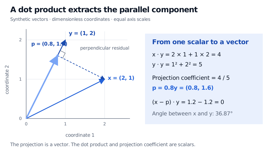
Take dimensionless vectors

\mathbf{x}=(2,1)^{\mathsf T}

and

\mathbf{y}=(1,2)^{\mathsf T}

. Their dot product is 4 and each squared Euclidean norm is 5, so

\cos\theta=4/5

and

\theta\approx36.87^\circ

To extract the part of

\mathbf{x}

along

\mathbf{y}

, use the orthogonal projection:

\mathbf{p} =\frac{\mathbf{x}\cdot\mathbf{y}}{\mathbf{y}\cdot\mathbf{y}}\mathbf{y} =\frac45\mathbf{y} =\begin{bmatrix}0.8\\1.6\end{bmatrix}.

The residual is $\mathbf{x}-\mathbf{p}=(1.2,-0.6)^{\mathsf T}$ . Its dot product with $\mathbf{y}$ is $1.2-1.2=0$ : everything remaining is perpendicular to the chosen direction.

Dimensionless vectors x=(2,1) and y=(1,2) have dot product 4 and angle 36.87 degrees. The projection p=(0.8,1.6) lies along y; the residual x−p=(1.2,−0.6) is perpendicular to y.

Original synthetic Euclidean example with equal axis scales. The dot product is a scalar; the projection is a vector.

The zero vector has dot product zero with every vector and is considered orthogonal to all of them. Its angle is undefined, and projection onto the zero vector is undefined because the denominator is zero. Projection of the zero vector onto a nonzero direction is the zero vector.

A change to a nonorthonormal basis requires accounting for the geometry of that basis; simply multiplying its new coordinates need not preserve the original Euclidean dot product. Likewise, scaling one financial feature from dollars to thousands changes raw geometric angles unless the metric or scaling convention compensates. A portfolio weight–return pairing is useful accounting; its angle is not a measure of portfolio quality.

Orthogonality does not establish independence

For two aligned, nonconstant return histories, subtract each series' own sample mean first. Writing the centred vectors as

\widetilde{\mathbf{x}}

and

\widetilde{\mathbf{y}}

, their Pearson correlation is

r_{xy}=\frac{\widetilde{\mathbf{x}}\cdot\widetilde{\mathbf{y}}} {\lVert\widetilde{\mathbf{x}}\rVert\lVert\widetilde{\mathbf{y}}\rVert}.

Thus centred orthogonal histories have zero sample correlation. Raw histories with a zero dot product need not. A constant history has zero centred length, so its correlation is undefined.

Even zero population covariance does not generally establish statistical independence. Let

U

take

-1,0,1

with equal probabilities, and set

V=U^2

. Their covariance is zero by symmetry, yet knowing

U

determines

V

. In particular, the chance of

V=0

1/3

before observing

U

, and 1 after observing

U=0

. Orthogonalising a factor removes a specified linear component; it does not remove every nonlinear relationship or prove that future losses are independent.

For a next step, Vectors and Matrices develops portfolio dot products into matrix calculations of factor exposures. The full lesson requires membership; a public preview is available.

Sources

Stephen Boyd and Lieven Vandenberghe, Introduction to Applied Linear Algebra: Vectors, Matrices, and Least Squares, §§1.4 and 3.4: weighted sums, portfolio value and return, angles and centred correlation. Author-hosted book and materials.
MIT OpenCourseWare, Calculus with Applications, §3.3, The Dot Product: the geometric identity and parallel/perpendicular decomposition.

A return calculation you can reconcile to cash

Matching entries is part of the model

Length, angle and the component in a direction

Orthogonality does not establish independence

Sources

Related terms

Basis

Correlation

Covariance

Euclidean norm

Independence

Orthogonal projection

Vector