Find the closest attainable vector, derive the projection formula, and distinguish Euclidean least squares from weighted risk metrics using a scenario P&L example.
Orthogonal projection
An orthogonal projection is the closest vector in a chosen subspace to a target vector, using a specified inner product to measure distance and perpendicularity. It separates the target into an attainable part and a residual perpendicular to every direction in that subspace. This is the geometry behind least squares: find the best approximation available from a restricted set of linear combinations.
For a trading desk, the distinction is practical. A target scenario P&L profile may be impossible to reproduce with the available instruments. Projection identifies the combination with the smallest squared mismatch under the chosen scoring rule. It does not make the mismatch disappear, or decide whether the scoring rule captures the desk's risk.
Which vector moves, and which set stays fixed?
Let y be the targetvector, and let U be the subspace of attainable fits. The projection p=PUy satisfies two conditions:
p∈U,r=y−p⊥U.
The first keeps the fit within the allowed set. The second says that the residual has zero inner product with every vector in that set. In ordinary Euclidean coordinates, the inner product is the dot product and distance is the Euclidean norm.
For a line through the origin with nonzero direction x, the attainable set is its span, U={ax:a∈R}. Write the fit as p=a^x. Orthogonality determines its coefficient:
x⊤(y−a^x)=0⟹a^=x⊤xx⊤y,p=x⊤xx⊤yx.
Here y stays fixed while ax moves along the line. Reversing target and direction asks a different question. Also distinguish the scalar coefficienta^ from the vector projectionp. Multiplying the direction by three divides its coefficient by three and leaves the fitted vector unchanged. If x=0, this formula divides by zero; projection onto the zero subspace itself is nevertheless well defined and equals zero.
A scenario fit with an unavoidable remainder
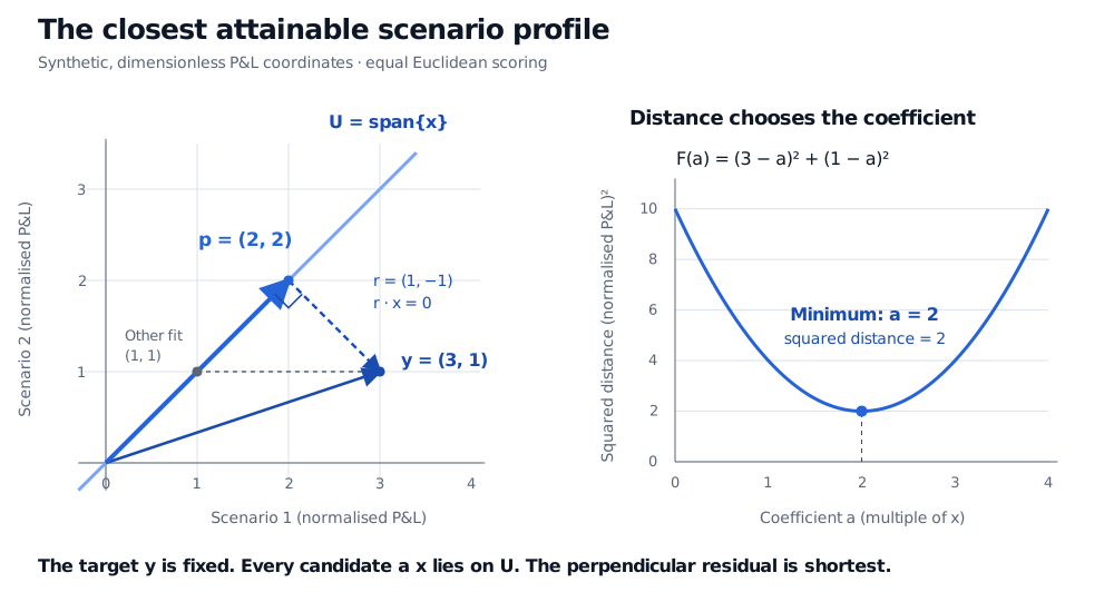
Consider an original synthetic example. A desk measures P&L in each of two alternative scenarios relative to the same reference amount, so both coordinates are dimensionless and commensurable. The target profile is y=(3,1)⊤. One reference quantity of the available instrument has profile x=(1,1)⊤. We assume P&L scales linearly with quantity, allow any real multiple, and give the two squared scenario errors equal weight. These scenarios are not a time series or probability forecast.
The instrument always produces equal scenario components, so no multiple can match both target components. Projection gives
a^=12+121×3+1×1=2,p=2x=(2,2)⊤,r=(1,−1)⊤.
The residual is perpendicular to the attainable line because x⊤r=1−1=0. The minimum distance is ∥r∥2=2 in normalised P&L units; its square is 2.
There is an independent way to see the optimum. The squared mismatch at any quantity multiple a is
F(a)=(3−a)2+(1−a)2=2(a−2)2+2.
The first term cannot be negative. It vanishes only at a=2, proving both the minimum and its uniqueness without relying on the projection formula.
Synthetic equal-weight scenario geometry: target y=(3,1) projects onto span of x=(1,1) at p=(2,2). The residual (1,-1) meets the line at a right angle. The squared-distance curve (3-a)²+(1-a)² has its unique minimum 2 at coefficient a=2.
Original synthetic scenario P&L example, expressed relative to one common reference amount. Left: a closest point in a vector space. Right: the same choice as minimisation over a scalar quantity. Equal weighting is a modelling assumption.
The coefficient 2 is a multiple of the instrument's reference quantity. It is not automatically a portfolio budget weight, a causal effect or an optimal trade after costs. Budget constraints, position limits and transaction costs would change the optimisation problem; a constrained attainable set need not be a subspace. Likewise, a best fit to two selected scenarios does not guarantee a good fit to other scenarios.
Why perpendicular means closest
For any competing fit u∈U, split its error into the orthogonal residual and an extra displacement within the subspace:
∥y−u∥22=∥r∥22+∥p−u∥22.
The cross term vanishes because r⊥U. Any departure from p therefore adds a nonnegative squared distance, with equality only at u=p. This establishes the closest-point property for any subspace of finite-dimensional Euclidean space, not just a line. In the example, the target's squared length also decomposes as 10=8+2: fitted part plus residual.
With several explanatory directions as columns of a matrixX, the fits are Xβ. Orthogonality becomes the normal equations:
X⊤(y−Xβ^)=0.
If the columns are independent, PU=X(X⊤X)−1X⊤. The projection matrix is symmetric and idempotent: PU⊤=PU and PU2=PU. A second projection changes nothing because the first fit already lies in U. Dependent columns still define a unique closest fitted vector, although different coefficients can describe that same vector. In computation, QR decomposition or SVD usually provides a better route than explicitly forming this inverse.
For ordinary least squares, these coordinates are observations: the response is projected onto the space spanned by the regressor columns. A regression with an intercept includes the constant vector in that space. Its residuals then sum to zero and have zero sample covariance with included regressors, in exact arithmetic. Without an intercept or appropriate centring, zero raw dot product alone does not imply zero sample covariance. In either case, orthogonality is an in-sample fitting property; it does not establish independence, causality or out-of-sample forecasting skill.
For a fuller derivation, Least Squares and Regression Geometry connects the projection, normal equations and an intercept-plus-factor return regression. Its public page provides a preview; the full lesson requires membership.
Change the metric, change the projection
Equal Euclidean weighting is a choice. Suppose the desk instead penalises the first scenario's squared error four times as heavily:
FW(a)=4(3−a)2+(1−a)2=5(a−513)2+516.
The optimum becomes a=13/5=2.6, giving fit (2.6,2.6)⊤ and residual (0.4,−1.6)⊤. That residual has ordinary dot product −1.2 with x, so it is not perpendicular in the ordinary plotted geometry. It is perpendicular under the weighted inner product⟨u,v⟩W=u⊤Wv, with W=diag(4,1):
x⊤Wr=4(0.4)−1.6=0.
More generally, a symmetric positive-definite W gives coefficient a^W=(x⊤Wy)/(x⊤Wx). A covariance-based risk criterion is another metric choice: a residual exposure vector e may be scored by e⊤Σe for a covariance matrix Σ. Generalised least squares instead uses an inverse error-covariance matrix when it exists. Neither is automatically the unweighted Euclidean problem. If the weighting matrix is only positive semidefinite, some nonzero directions can have zero measured length, so the usual positive-definite uniqueness argument needs reconsideration.
Before calling a projection the “best hedge” or “best explanation”, state the target, attainable subspace, coordinate units and loss metric. That is what makes the geometry an economic model rather than a picture.
Sources
Gilbert Strang, Introduction to Linear Algebra, 5th edition, Wellesley–Cambridge Press, 2016, §4.2 “Projections” and §4.3 “Least Squares Approximations”.