Ordinary least squares minimises squared residuals. Fit a factor-return line, track intercept and slope units, and separate rank, inference and causal assumptions.
Ordinary least squares
Ordinary least squares (OLS) estimates the coefficients of a linear regression by minimising the sum of squared differences between observed responses and fitted values. Each observation receives equal weight. In a return regression, this gives a reproducible answer to “which factor exposure and intercept fit these observations best under squared error?” It does not, by itself, establish why returns moved or whether the fitted relationship will persist.
Linear regression describes the model; OLS is a method for fitting its coefficients. “Linear” means linear in those coefficients: a model using predetermined squared or transformed predictors can still be fitted by OLS. NIST explains this distinction.
What the fit minimises
For observations (xi,yi), a simple line with an intercept has fitted values and residuals
The residual is a vertical difference in the response variable's units, evaluated at the observed xi. OLS does not minimise perpendicular distances to the line, and exchanging response and predictor generally produces a different fit. Squaring prevents positive and negative misses from cancelling and makes large misses particularly influential. Equal weighting distinguishes ordinary least squares from weighted least squares.
Let xˉ and yˉ be the sample means. Provided the predictor values are not all equal,
Consider these synthetic monthly excess returns, with the asset and factor measured over the same months and with the same risk-free-return convention. Both columns are recorded in percentage points (pp): an entry of 1 means a return of 1%, or 0.01 in decimal-return units.
Month
Factor xi (pp)
Asset yi (pp)
Fitted y^i (pp)
Residual ei (pp)
Squared residual (pp²)
1
−1.0
−0.8
−0.9
+0.1
0.01
2
0.0
0.1
0.3
−0.2
0.04
3
1.0
1.6
1.5
+0.1
0.01
The means are xˉ=0 and yˉ=0.3. The centred predictor squared sum is 2 pp², and the centred cross-product sum is 2.4 pp². Hence
b^=22.4=1.2,a^=0.3 pp,y^=0.3+1.2x.
The residual sum of squares, also called SSE or RSS, is
SSE=0.12+(−0.2)2+0.12=0.06 pp2.
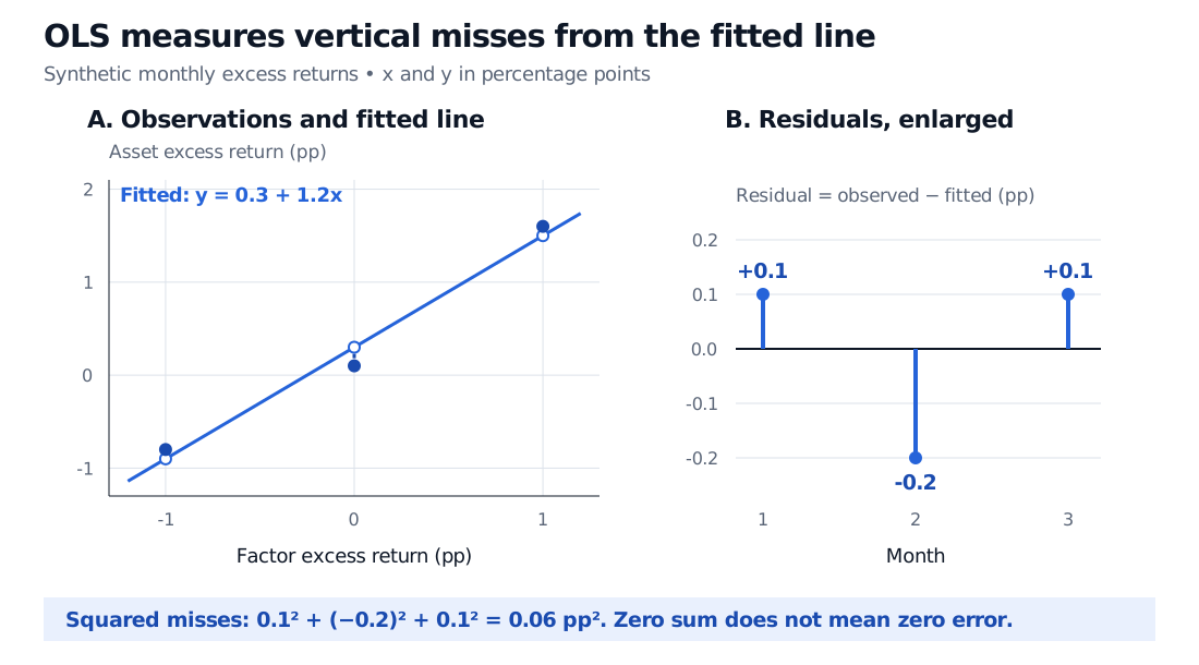
The middle observation has the largest miss and contributes two-thirds of SSE. Positive residuals mean that the asset return exceeded the line's fitted value; they do not mean that the asset made a positive return. Month 1 has a positive residual despite its negative asset return.
Synthetic monthly factor and asset excess returns in percentage points. The fitted line is y = 0.3 + 1.2x; fitted asset returns are −0.9, 0.3 and 1.5. The enlarged residual panel shows +0.1, −0.2 and +0.1 pp, whose squared sum is 0.06 pp².
Original synthetic example. Panel A shows vertical differences from the fitted line; panel B enlarges the residual scale. All return axes use percentage points.
The slope says that a one-percentage-point increase in the factor corresponds to a 1.2-percentage-point increase in the fitted asset return. If this factor is the market's excess return, the slope is the sample market beta. It measures fitted factor sensitivity; it does not alone determine the asset's total volatility.
The intercept is the fitted monthly asset excess return when the factor excess return is zero. It equals the sample mean here because xˉ=0; that equality is not universal. A factor-regression intercept is often called estimated alpha, but these three constructed observations establish no economic alpha, persistent skill or abnormal future return.
Units must travel with the coefficients. Converting both return columns to decimals gives intercept 0.003, unchanged slope 1.2, and SSE 0.000006 in decimal-return squared units. The factor 10,000 between the two SSE numbers comes from squaring the unit conversion. The intercept is a monthly quantity; OLS has not annualised it.
Why the minimum and the intercept matter
Differentiating the objective with respect to the intercept and slope gives the normal equations, expressed through the fitted residuals:
i∑ei=0,i∑xiei=0.
Both hold in the example. They are identities created by the fit, rather than evidence that the underlying economic errors have zero conditional mean. In particular, a zero average residual is guaranteed by an unconstrained OLS intercept even for a badly specified model.
There is a direct minimum certificate for these three observations. Move the intercept from 0.3 to 0.3+u and the slope from 1.2 to 1.2+v, using the same percentage-point input convention. Expanding the squares and using the two residual identities gives
Q(0.3+u,1.2+v)=0.06+3u2+2v2.
Every coefficient change raises the objective unless both changes are zero. The fitted line therefore has the unique global minimum for this dataset.
Removing the intercept changes the problem. Here a line forced through zero still has slope 1.2, but SSE rises to 0.33 pp² and the residuals no longer sum to zero. Subtracting a risk-free rate from both return series does not automatically justify forcing the factor regression through the origin.
Several factors: uniqueness belongs to the design
For several predictors, collect the response observations into y and the predictor columns into the design matrix X. Include a column of ones if the model has an intercept. OLS solves
βmin∥y−Xβ∥2,X⊤(y−Xβ^)=0.
The fitted vector is the orthogonal projection of y onto the column space of X. Coefficients are unique when X has full column rank. In that case the formal expression is
β^=(X⊤X)−1X⊤y.
A numerical least-squares solver based on QR or SVD is generally preferable to explicitly forming that inverse. Nearly redundant columns can make coefficients unstable even when exact rank is full.
If columns are exactly redundant, coefficient vectors need not be unique, while the fitted values for the observed design remain unique. For a constant predictor xi=c, only the combination a+bc is identified. This is why the simple-line formula requires nonzero predictor variation; more rows alone cannot repair a rank-deficient design.
From fitting to inference or causation
A calculated line is an in-sample summary. Each stronger interpretation requires more:
Conditional mean. To treat the population line as E[Y∣x]=a+bx, specify a linear conditional expectation, equivalently a zero conditional-mean error for that model. A best linear approximation need not equal a nonlinear conditional mean.
Uncertainty. Under a full-rank correctly specified model with zero-mean errors conditional on the design, constant conditional variance and zero cross-observation error covariance give the classical coefficient covariance formula. Independent normal errors conditional on the design additionally justify exact finite-sample normal and Student-t inference. Normal returns are not a requirement for merely fitting OLS.
Financial time series. Heteroskedasticity and autocorrelation can invalidate classical standard errors. Robust or HAC methods address particular covariance problems under their own sampling conditions; they do not cure endogeneity, poor specification or an inadequate sample.
Causation. A causal coefficient needs an identification argument, such as a defensible assignment mechanism and control of confounding. Minimising squared residuals supplies none of that argument.
This example has only n−2=1 residual degree of freedom. It cannot meaningfully diagnose the assumptions needed for an economic claim. In real work, align observations and units, inspect influential points and residual patterns, and evaluate stability on data outside the fitting sample. An unusually large miss receives substantial weight under squared error, as NIST's discussion of outlier sensitivity warns.
For a first hand calculation, Basic Statistics and Regression is available in full with a free signed-in account. For the derivation, projection geometry and classical coefficient inference, read Linear Regression; its full lesson requires membership, with a public preview.
Sources
John A. Rice, Mathematical Statistics and Data Analysis, 3rd edition, §§14.1–14.2.1: vertical least-squares criterion, coefficient formulas and statistical assumptions; §14.3: normal equations, rank and matrix formulation. The returns, calculations and figure above are original.