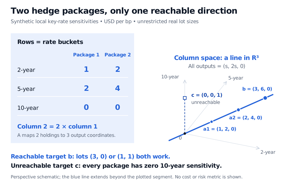
The column space is the set of outputs a matrix can reach. Use a three-bucket hedge example to distinguish coverage, rank, nonunique holdings and trading constraints.
Column space
The column space of a matrix is the set of every output that matrix can produce when multiplied by an unrestricted input vector. If the columns describe instrument exposures and the inputs are holdings, the column space answers a practical question: which exposure targets can this instrument set deliver?
For a real m×n matrix A=[a1⋯an],
C(A)={Ax:x∈Rn}=span{a1,…,an}⊆Rm.
Here span means all linear combinations of the columns. Each column has m entries, so the column space lives in the output spaceRm, even though there are n columns. It is a subspace: it contains zero and is closed under addition and real scaling. Strang's Introduction to Linear Algebra, §3.1, develops this output-space interpretation.
Two packages cannot necessarily cover three rate buckets
A desk can adjust positions in two hypothetical hedge packages. Their signed local sensitivities to the 2-year, 5-year and 10-year yield-curve buckets are the columns of
A=120240.
Rows are rate buckets; columns are packages. Each entry is the change in package value, in USD per basis-point increase in that bucket's yield, per lot, at a fixed valuation point and under a specified curve-bump convention. Positive entries mean a gain when that yield rises. These are synthetic signed sensitivities, rather than observed bond prices or a claim about a standard DV01 sign convention.
Let x=(x1,x2)⊤ be real-valued lot holdings, with negative holdings representing shorts. The resulting sensitivity vector is
Ax=x1+2x22x1+4x20=(x1+2x2)120.
The second package supplies twice the first package's sensitivity profile. It changes how a target can be implemented, but adds no new output direction. Thus
C(A)={(s,2s,0)⊤:s∈R}.
This is a line inside a three-dimensional output space. Its dimension is one, which is the rank of A. Two available packages do not imply two independent directions of hedge coverage.
Consider a desired sensitivity change b=(3,6,0)⊤, measured in USD per bp in the same bucket order. Both of these holdings achieve it:
Package 1 lots
Package 2 lots
Resulting sensitivity, USD per bp
3
0
(3,6,0)
1
1
(3,6,0)
Indeed, every x=(3−2t,t)⊤ with t∈R gives this target. Moving between those holdings adds a multiple of (−2,1)⊤, a null-space direction that changes positions while leaving the measured sensitivities unchanged.
By contrast, c=(0,0,1)⊤ is unreachable. The third component of Ax is always zero, so no position sizes can generate the requested 10-year sensitivity. Nor is zero third-bucket exposure sufficient for reachability: the first two components must also satisfy b2=2b1.
A synthetic three-by-two sensitivity matrix has columns (1, 2, 0) and (2, 4, 0), in USD per bp per package lot. Their column space is one line in three output coordinates. Target (3, 6, 0) is reached by lots (3, 0) or (1, 1); target (0, 0, 1) lies outside that line.
Original synthetic local-sensitivity example. The perspective drawing shows a line in three dimensions; its displayed segment continues in both directions. All output components use USD per bp.
These calculations concern local linear sensitivity matching. They do not establish exact payoff replication for large yield moves: curvature, changing sensitivities and unmodelled curve movements can leave residual P&L.
Reachability and uniqueness are separate questions
A system of linear equationsAx=b has a solution if and only ifb∈C(A). That says whether a target is reachable. It does not say whether the holdings are unique.
For an m×n matrix of rank r:
Every output target is reachable exactly when r=m, so C(A)=Rm.
Each reachable target has unique holdings exactly when r=n, so the null space contains only zero.
Our example has r=1<m=3 and r=1<n=2: some targets are impossible, while every reachable target has infinitely many unrestricted holdings.
The row space belongs to the input-coordinate space R2 here: it is generated by (1,2). The column space belongs to R3: it is generated by (1,2,0). They have equal dimension—rank one—but are different spaces with different jobs. A row computes one bucket's sensitivity from holdings; the columns determine which complete sensitivity profiles can be produced.
To find a column-space basis by elimination, locate the pivot columns and then take the corresponding original columns of A. Row operations preserve rank but can change the column space itself. In this example the first original column alone is a basis.
A reachable target still needs an executable trade
Column-space membership allows arbitrary real coefficients. A desk may face lot-size rules, short-sale restrictions, position caps, funding limits and transaction costs. Those restrictions can remove holdings that the algebra permits. If allowed holdings form a set F, the practically admissible outputs are {Ax:x∈F}, generally only a subset of C(A).
Even the two portfolios in the table can have different purchase costs, liquidity and omitted risks. Rank supplies a statement about independent measured output directions; it supplies no price, financing plan or guarantee of a costless hedge. Adding another package enlarges the column space only if its column lies outside the existing space. A duplicate profile may still help execution, but cannot cure missing mathematical coverage.
For a longer treatment connecting holdings, attainable targets and null-space freedom, see Vectors, Matrices and Linear Systems. The public page provides a preview; the full lesson requires membership.
Sources
Gilbert Strang, Introduction to Linear Algebra, 5th edition, §3.1, “Spaces of Vectors,” especially “The Column Space of A”; §3.5, “Dimensions of the Four Subspaces.”