A subspace contains zero and is closed under addition and all real scaling. Build a dollar-neutral portfolio plane and distinguish it from a fully invested budget.
Subspace
A subspace is a subset of a vector space that is itself a vector space under the same addition and scalar multiplication. In a real vector space, it contains zero and stays closed when its vectors are added or multiplied by any real number.
For a portfolio desk, this identifies constraints that survive combining books, reversing their signs and changing their size. A zero net dollar-exposure constraint has this structure. A requirement that portfolio weights sum to one does not: it defines a shifted, affine set. Both are useful, but they permit different combinations.
The three-part test
For a subset S of a real vector space V, check:
Zero:0∈S.
Addition: if u,v∈S, then u+v∈S.
All real scaling: if v∈S and c∈R, then cv∈S.
The other vector-space laws are inherited from V. Equivalently, a nonempty subset is a subspace if every linear combinationau+bv stays inside it. Negative coefficients matter: closure only under positive scaling is insufficient. Axler's subspace criterion, §1C, result 1.34, formalises this test.
Passing through the origin is necessary, but alone proves little. The union of the two coordinate axes contains zero, yet (1,0)+(0,1)=(1,1) leaves that union. In contrast, {0} and the whole ambient space V are always subspaces. The empty set is not.
Three assets, two independent dollar-neutral trades
Fix a common reference amount of USD 1 million. Define wi as the signed marked dollar exposure to asset i divided by that reference: positive for long, negative for short. These are exposure fractions, not share counts or weights divided by a zero net portfolio value. Assume unrestricted real positions for the algebra.
The dollar-neutral set is
S={w∈R3:w1+w2+w3=0}.
Zero belongs. If two books each sum to zero, their sum does too; multiplying either by any real c gives component sum c⋅0=0. Thus S is a subspace.
Two useful trading directions are
b1=(1,−1,0),b2=(1,0,−1).
Every neutral exposure has the form
ab1+bb2=(a+b,−a,−b),a,b∈R.
To see that this reaches every member of S, set a=−w2 and b=−w3. Neutrality then supplies w1=−w2−w3=a+b. The representation is unique: its second and third entries determine a and b separately. These two directions therefore form a basis for S, and its dimension is two. It is a plane inside the three-coordinate ambient space, rather than all of R3.
For example,
w=(0.6,−0.2,−0.4)=0.2b1+0.4b2
means long USD 600,000 of asset 1 and short USD 200,000 and USD 400,000 of assets 2 and 3. Combining it with z=(−0.1,0.3,−0.2) gives (0.5,0.1,−0.6), still neutral. Reversing and doubling the original gives −2w=(−1.2,0.4,0.8), also neutral.
All books must use the same reference amount for this componentwise addition to describe their combined exposures. Adding weights independently normalised to different account sizes does not directly add the underlying dollars.
Dollar neutrality removes one exposure measure. It does not imply zero market beta, zero variance, zero funding need or a profitable trade. Short-sale proceeds, collateral, margin, borrow availability and costs require their own treatment. This static equality also does not by itself establish that a dynamic trading strategy is self-financing.
Why a budget behaves differently
Now require
F={w∈R3:w1+w2+w3=1}.
Under the same reference convention, this fixes net marked exposure at USD 1 million. When the reference is portfolio capital and these assets account for the entire allocation, it is the usual fully invested budget constraint, allowing shorts unless separately forbidden.
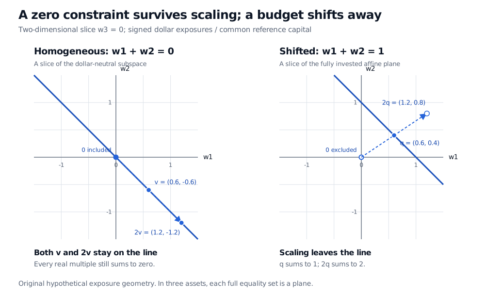
Zero is absent, so F is not a subspace. The feasible book q=(0.6,0.4,0) sums to one, whereas 2q=(1.2,0.8,0) sums to two. Adding two feasible books has the same problem.
On the slice w3 equals zero, the dollar-neutral line contains zero, v=(0.6,-0.6) and 2v=(1.2,-1.2). The shifted budget line contains q=(0.6,0.4), but excludes zero and 2q=(1.2,0.8). Coordinates are signed dollar exposures divided by common reference capital.
Original hypothetical exposure geometry. The diagram fixes the third exposure at zero; the full sets in three assets are planes. Dashed arrows show scaling from the origin, with equal axis scales.
There is still useful linear structure. Choose q0=(1,0,0). Then
F=q0+S.
This is an affine plane: a translation of the neutral subspace. The difference between any two fully invested allocations belongs to S. Rebalancing within a fixed budget therefore uses zero-net-exposure increments. Also, λu+(1−λ)v remains in F whenever u,v∈F; its coefficients add to one. For 0≤λ≤1, this describes a mixture of allocations.
Homogeneous constraints reveal the general pattern
is a subspace, called its null space. Matrix linearity preserves the zero right-hand side under addition and scaling. Our example uses the single row A=[111]. Several fixed linear neutrality requirements can be stacked as rows; their common solution set is still a subspace. Dependent rows need not remove further dimensions.
A nonempty solution set Aw=b with b=0 is instead a translate of the null space. Inequalities require a separate check. The long-only orthant contains (1,0,0) but excludes its negative. An exposure cap ∣wi∣≤0.75 admits our original neutral book, but excludes its doubled version. Such feasible sets generally fail subspace closure. One special case is worth keeping straight: dollar neutrality and nonnegative exposures together force every exposure to zero, leaving the valid trivial subspace {0}.
The span of any collection of vectors is always a subspace. A feasible investment mandate need not be. Before applying an unrestricted linear solve or combining hedges, identify which constraints are homogeneous equalities and which introduce budgets, bounds or trading restrictions.
Vector Spaces and Subspaces develops the closure test and its geometric counterexamples. The Nullspace — Solving Ax = 0 shows how row reduction constructs the directions satisfying multiple homogeneous equations. Both have public previews; full lessons require membership.