Dimension counts the independent coordinates needed to describe an object within a specified mathematical space. For a finite-dimensional real vector space, it is precisely the number of vectors in any basis. A portfolio can store three asset weights while leaving only two independent allocation choices: a budget equation determines the third.
The basis may change, but its size does not. MIT's Independence, Basis and Dimension session develops this connection between spanning a space and removing redundant directions. Dimension is a property of the space being described, rather than the length of a particular list of instruments.
Three weights do not always mean three choices
Consider a synthetic portfolio with real-valued weights
Each weight is a fraction of portfolio net asset value. Before imposing restrictions, the ambient dimension is three: the surrounding coordinate space is . Negative weights are allowed at this stage.
A fully invested budget constraint requires
Choose and freely; then . Equivalently,
The two adjustment directions are linearly independent, so the budget leaves two degrees of freedom. All vectors still contain three entries. The allowed set is a two-dimensional affine plane inside a three-dimensional ambient space.
An affine plane is a shifted vector subspace. This budget plane is not itself a vector subspace: it excludes the zero vector, and adding two fully invested weight vectors produces weights summing to two. Its dimension is the dimension of its parallel adjustment subspace. Boyd and Vandenberghe, §2.1.2, formalise this affine-set distinction.
Now require zero exposure to one toy factor whose asset loadings are :
This is a second, independent equation. Together the equations give
The matrix rank is two. Setting yields the complete family
There is one free parameter. For example, gives , with budget one and factor exposure zero. This is neutrality to the specified factor only; it does not eliminate all financial risk.
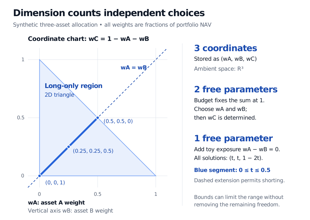
Original synthetic allocation example. Axes show asset A and B weights, each a fraction of NAV; the third weight is 1 minus their sum. The filled triangle adds long-only bounds. The dashed line extends the exposure-neutral family when shorting is allowed.
Count independent restrictions, then check feasibility
For a consistent real linear system with unknowns,
This is an affine dimension. A particular solution supplies the offset; the null space supplies the directions along which it can vary. With a zero right-hand side, the solution set is itself a vector subspace.
Two checks prevent the usual counting errors:
- Repeated equations do not remove extra freedom. Adding to the budget adds a row but leaves rank one and dimension two.
- Contradictory equations remove every solution. Replacing that right-hand side by three conflicts with the budget. The feasible set is empty; reporting as its dimension would misdescribe the problem. Check consistency before applying the formula.
Inequalities need their own examination. Adding bounds the budget plane to a filled triangle whose affine dimension remains two. Adding these long-only bounds to the exposure-neutral line restricts to : a one-dimensional segment. Endpoints do not make the whole segment zero-dimensional.
Bounds can also collapse the set. Budget one, long-only weights and together force , a single point of affine dimension zero. Thus “an inequality never changes dimension” is false.
For these nonempty convex feasible sets, affine dimension means the dimension of the smallest affine set containing them, their affine hull. This is the convention in Boyd and Vandenberghe, §2.1.3. General nonlinear sets require care: their intrinsic dimension need not equal their affine dimension.
Coordinate count, matrix shape and rank answer different questions
A matrix can map three input coordinates to two output coordinates while producing only one independent output direction. For example,
| Count | Value here | What it describes |
|---|---|---|
| Input ambient dimension | 3 | Coordinates in each input vector |
| Output ambient dimension | 2 | Coordinates in each output vector |
| Rank | 1 | Dimension of the reachable output space |
Counting assets, columns or reported exposures alone does not establish the dimension of their span. In a numerical application, near dependence also requires a stated tolerance and sensible scaling; the exact ranks above concern the stated exact coefficients.
Finally, physical dimension has a different meaning: currency, time or currency per share describe units, rather than the number of independent directions. A one-dimensional price variable can carry USD units; portfolio weights can be dimensionless fractions while ranging over a two-dimensional feasible set.
For the basis argument and payoff-space examples, see Linear Independence, Basis, and Dimension. For offsets, null-space freedom and consistency, see The Complete Solution to Ax = b. Both have a public preview; their full lessons require membership.
Sources
- Gilbert Strang, Introduction to Linear Algebra, 5th ed., §§3.3–3.5: complete linear-system solutions, basis, dimension and dimensions of matrix subspaces.
- MIT OpenCourseWare, Independence, Basis and Dimension, 18.06SC: basis size and dimension, with lecture and worked materials.
- Stephen Boyd and Lieven Vandenberghe, Convex Optimization, Cambridge University Press, 2004, §§2.1.2–2.1.3: affine sets, their direction subspaces, affine hulls and affine dimension.