Null space: Definition & Examples

The null space of a matrix is the set of input vectors that it maps to zero. For a real

m\times n

matrix

A

N(A)=\ker(A)=\{\mathbf{x}\in\mathbb{R}^n:A\mathbf{x}=\mathbf{0}\}.

It is also called the kernel of the matrix. In a portfolio exposure model, it answers a useful question: which changes in positions leave every measured exposure unchanged? A nonzero answer can give a desk room to change inventory while preserving a hedge. It does not mean the position has disappeared or that every economic risk has been hedged.

The distinction between input and output matters.

N(A)

lives in the input space

\mathbb{R}^n

, where positions are recorded. The zero on the right is in the output space

\mathbb{R}^m

, where the measured exposures are recorded. The column space instead describes which outputs can be reached.

A book that vanishes from two exposure reports

Consider three hypothetical cash instruments and two modelled return factors. Their dimensionless factor loadings are

A=\begin{pmatrix}1&1&0\\0&1&1\end{pmatrix}.

Columns correspond to instruments A, B and C; rows to factors 1 and 2. Let

\mathbf{w}

give signed current market values in USD millions, with a negative entry representing a short position. Then

A\mathbf{w}

gives the two factor exposures in USD millions: each exposure multiplied by its factor's decimal return contributes P&L in USD millions under this linear model.

The book

\mathbf{w}=\begin{pmatrix}1\\-1\\1\end{pmatrix} \quad\text{gives}\quad A\mathbf{w}=\begin{pmatrix}1-1+0\\0-1+1\end{pmatrix} =\begin{pmatrix}0\\0\end{pmatrix}.

Long USD 1 million of A and C and short USD 1 million of B cancel both reported factor exposures. Equivalently, B's loading column is the sum of A's and C's columns. The columns are linearly dependent, so different position vectors can produce the same exposure report.

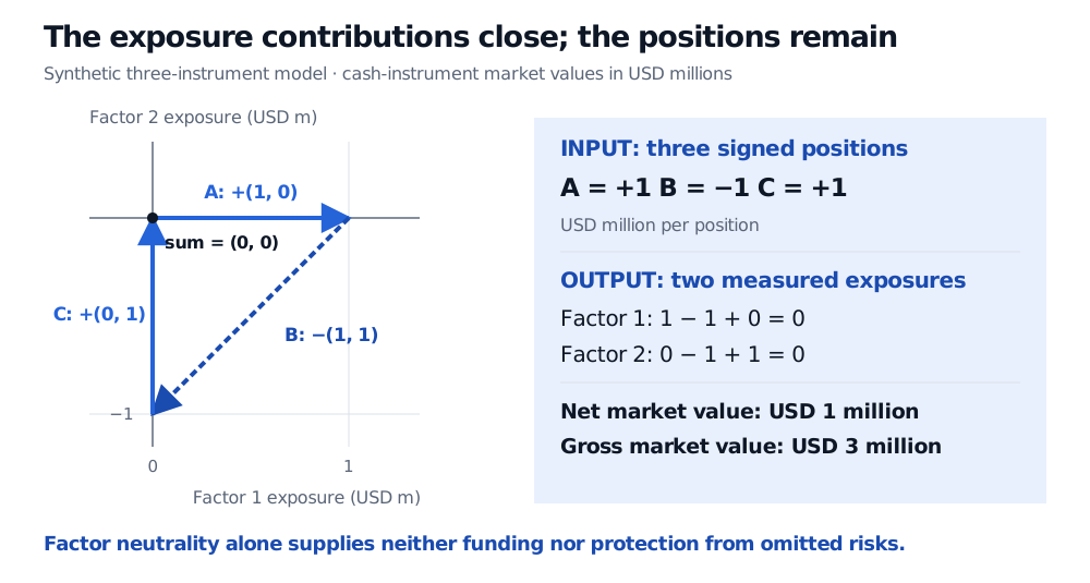
In a synthetic model, signed exposure contributions (1,0), (-1,-1) and (0,1), in USD millions, form a closed triangle. Positions (1,-1,1) still have USD 1 million net market value and USD 3 million gross market value.

Original synthetic factor-loading example. The arrows lie in the two-dimensional exposure space; the null vector itself has three position components. Equal axis scales show the cancellation. Neither factor is a complete account of risk.

Zero measured exposure is not zero investment. This book has net market value

1-1+1=\text{USD }1

million and gross market value

1+1+1=\text{USD }3

million. A financing trade is still needed to establish a zero-initial-outlay package, and financing can bring its own costs and constraints.

Zero measured exposure is not zero P&L either. For example, suppose the instruments have residual returns

(1\%,0,0)

after their modelled factor contributions. This book earns USD 10,000 from those residuals, regardless of the cancelled factor contribution. Other residual outcomes can lose money. Idiosyncratic risk, omitted factors, changing loadings, short borrow and trading costs survive the equation. A null vector of a factor-loading matrix is therefore insufficient to establish an arbitrage.

Find all the directions, not just one lucky cancellation

Solving $A\mathbf{x}=\mathbf{0}$ gives

x_1+x_2=0,\qquad x_2+x_3=0.

Subtract the second matrix row from the first. The reduced row echelon form is

R=\begin{pmatrix}1&0&-1\\0&1&1\end{pmatrix}.

Elementary row operations preserve the solution set of the homogeneous system. Columns 1 and 2 contain pivots;

x_3

is free. Setting

x_3=t

forces

x_1=t

and

x_2=-t

, so the entire null space is

N(A)=\left\{t\begin{pmatrix}1\\-1\\1\end{pmatrix}:t\in\mathbb{R}\right\}.

The single vector

(1,-1,1)^\top

is a basis for this null space. Setting

t=0

gives the zero book; negative

t

reverses the positions. This is a line through the origin in three-dimensional position space, even though the exposure chart above is two-dimensional.

More generally, row-reduce $A$ , identify the free variables, and construct one solution for each free variable by setting it to one and the others to zero. Those solutions form a null-space basis. The rank–nullity theorem counts the directions:

\dim N(A)=n-\operatorname{rank}(A).

Here the first two columns form an invertible

2\times2

block, so the matrix rank is two and nullity is

3-2=1

. Count columns, rather than rows, in this subtraction.

The null space is always a subspace: it contains zero, and adding or scaling zero-output inputs still gives zero output. It is never empty. A matrix with full column rank has the trivial null space

\{\mathbf{0}\}

; a zero matrix maps every input to zero and has the whole input space as its null space.

The same hedge, with different inventory

Suppose the desired exposures are $\mathbf{b}=(2,1)^\top$ in USD millions. One solution is $\mathbf{w}_p=(2,0,1)^\top$ . Every solution is

\mathbf{w}=\mathbf{w}_p+t\begin{pmatrix}1\\-1\\1\end{pmatrix} =\begin{pmatrix}2+t\\-t\\1+t\end{pmatrix}.

For example, $(1,1,0)$ , $(2,0,1)$ and $(3,-1,2)$ all deliver exposures $(2,1)$ . The factor report alone cannot choose among them; financing, residual risk, liquidity, costs and position limits may do so.

This is a translated, or affine, copy of the null space. Since

\mathbf{b}\ne\mathbf{0}

, it does not pass through zero and is not itself a vector subspace. In general, a target outside the column space has no solution. When a solution exists, the difference between any two solutions lies in

N(A)

, because subtracting their equations gives

A(\mathbf{w}_1-\mathbf{w}_2)=\mathbf{0}

Constraints can remove the freedom. In the zero-factor-exposure example, additionally requiring zero net market value means $x_1+x_2+x_3=0$ . Along the null line that sum equals $t$ , so only $t=0$ satisfies all three conditions. A budget row must be included explicitly if it is part of the intended hedge.

Exact algebra and estimated loadings

An exact null space belongs to the specified matrix. With estimated loadings, $A\mathbf{w}=0$ means neutrality to those estimates. It does not promise that realised exposures are zero.

For computation, row reduction explains the structure; a singular value decomposition can identify exact or approximate null directions numerically. A tiny output can indicate an approximate cancellation, but the numerical rank depends on the stated tolerance and scaling. Different factor units or rounded coefficients can change that diagnosis. Large offsetting positions can also magnify small loading errors.

For the systematic free-variable construction, see The Nullspace: Solving Ax = 0. For holdings, attainable targets and the separate financing condition, see Vectors, Matrices and Linear Systems. Both offer public previews; the full lessons require membership.

Sources

Gilbert Strang, Introduction to Linear Algebra, 5th edition, Wellesley–Cambridge Press, 2016, §3.2, “The Nullspace of A: Solving Ax = 0 and Rx = 0”; §3.3, “The Complete Solution to Ax = b.” Definitions, free-variable construction, rank and complete-solution geometry. All financial examples and the figure here are original.
MIT OpenCourseWare, Gilbert Strang, Solving Ax = 0: Pivot Variables, Special Solutions — 18.06SC, Fall 2011, session on elimination, pivots and null spaces, with lecture summary and exercises.

A book that vanishes from two exposure reports

Find all the directions, not just one lucky cancellation

The same hedge, with different inventory

Exact algebra and estimated loadings

Sources

Related terms

Arbitrage

Basis

Column space

Idiosyncratic risk

Linear dependence

Matrix

Matrix rank

Subspace