A basis spans a specified vector space without redundant directions. Decompose a two-tenor yield shock, distinguish coordinates from vectors, and interpret factor units.
Basis
A basis for a vector space is a collection of vectors that both spans that space and is linearly independent. Spanning means every vector in the space can be built from them; independence means the representation contains no redundant direction. Once the basis and its order are fixed, every vector has exactly one set of coordinates. Axler's basis criterion states this equivalence formally in §2B, result 2.28.
For a risk analyst, a basis can turn a list of yield changes into interpretable level and tilt amplitudes. The underlying shock stays the same; the numbers used to describe it change. Here basis means the linear-algebra concept, rather than the cash–futures price difference used when discussing basis risk.
Why both conditions matter
For a finite ordered basis B=(b1,…,bk) of a real vector space V, every v∈V has a unique linear combination
v=c1b1+⋯+ckbk.
The coefficient column [v]B=(c1,…,ck)T is its coordinate vector relative to this ordered basis.
The two requirements do different jobs:
Span gives existence. Without it, some targets cannot be reached.
Linear independence gives uniqueness. If two coefficient lists produced the same target, subtracting their representations would give a zero combination. Independence forces every coefficient difference to be zero.
Always name the space. The single vector (1,1) is a basis for the line L={(t,t):t∈R}, but cannot span the whole plane R2. Adding (2,2) still reaches only that line and introduces redundancy: (2,2)=2(1,1). These two vectors are therefore not a basis even for L. A basis of a finite-dimensional space has as many vectors as the space's dimension.
One yield shock, two descriptions
Suppose a hypothetical yield curve has just two observed tenors, ordered short first, long second. Its change is +3 basis points at the short tenor and +1 basis point at the long tenor. In ordinary tenor coordinates,
v=[31] bp.
Choose the dimensionless shapes
b1=[11],b2=[1−1].
The first is a parallel level direction. A positive amplitude of the second raises the short yield and lowers the long yield; call it tilt here. Under the long-minus-short definition of slope, that positive tilt reduces slope. Names alone do not determine signs.
Reading the two rows gives c1+c2=3 bp and c1−c2=1 bp. Adding and subtracting yields
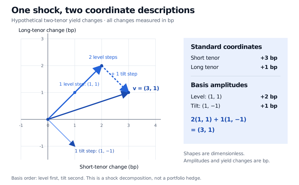
c1=2 bp,c2=1 bp,v=(2 bp)b1+(1 bp)b2.
Thus the same shock has tenor coordinates (3,1) bp and basis coordinates (2,1) bp. The determinant is 1(−1)−1(1)=−2=0, so these columns form a basis for the entire two-tenor plane, not just for this particular shock.
A hypothetical yield shock has short-tenor change 3 bp and long-tenor change 1 bp. A solid blue path takes two level steps to (2,2), then a dashed tilt step reaches (3,1). Its basis amplitudes are 2 bp level and 1 bp tilt.
Original hypothetical two-tenor example. Dimensionless basis shapes; both yield changes and their amplitudes are in basis points. Equal plot scales show the actual vector construction.
More generally, a shock (x,y) bp has amplitudes
[v]B=[(x+y)/2(x−y)/2] bp.
This is a change of basis, with B mapping basis amplitudes into tenor changes. Reversing the order of the basis reverses the order of the coordinates. Doubling the level shape to (2,2) halves its coefficient: this same shock then needs 1 bp of the new level amplitude and 1 bp of tilt. Coordinate values require the basis's order, scale and units to be meaningful.
A basis need not be orthonormal
Our chosen shapes happen to be perpendicular under the ordinary Euclidean dot product, since 1(1)+1(−1)=0. Each has length 2, so this basis is orthogonal but not orthonormal. Orthonormality adds unit lengths; neither perpendicularity nor unit length is required for a basis. For example, (1,0) and (1,1) are not perpendicular but do form another basis of the plane.
For a general square basis matrix, coordinates solve Bc=v; they are not automatically the dot products biTv. Even here, those dot products give (4,2) bp and must each be divided by the corresponding squared length, 2, to recover (2,1) bp. The unadjusted dot-product rule works for an orthonormal basis.
What the decomposition does—and does not—tell a desk
This example decomposes yield changes, not holdings. Its amplitudes are not investment weights and need not add to one. To translate a yield shock into approximate P&L, a desk also needs sensitivities with matching tenor definitions, signs and currency-per-bp units. To construct trades, it needs an instrument-exposure map and trading constraints. A basis by itself supplies neither prices nor an executable hedge.
Two tenors give a complete two-dimensional description only of those two entries. They cannot capture an independent third-tenor move. Similarly, linearly independent factor shapes need not be statistically independent random factors, and a historical low-dimensional fit need not exactly span future shocks.
Finally, exact independence does not guarantee reliable numerical coordinates. Nearly parallel shapes can form a valid basis while making the solve sensitive to small input errors. A nonzero determinant establishes the exact algebraic result; numerical conditioning, input scaling and any rank tolerance still matter in a computed risk report.
Gilbert Strang, Introduction to Linear Algebra, fifth edition (Wellesley-Cambridge Press, 2016), §3.4, “Independence, Basis and Dimension.” See also MIT OpenCourseWare Lecture 9.
Sheldon Axler, Linear Algebra Done Right, second edition (Springer), Chapter 2, “Bases,” pp. 27–28, Proposition 2.8.