A linear combination scales vectors and adds them. Build a two-state claim payoff, distinguish contract quantities from probabilities, and separate replication from pricing.
Linear combination
A linear combination is a vector formed by multiplying given vectors by scalar coefficients and adding the results. For real vectors v1,…,vk in the same vector space, it has the form
y=c1v1+⋯+ckvk,ci∈R.
Each coefficient scales an entire vector. Addition then combines corresponding components. Coefficients may be positive, zero or negative; the definition does not require them to sum to one. This is the operation behind adding trading positions, combining factor exposures and constructing a target cash flow. Axler's definition gives the general vector-space formulation.
Two claims, two alternative states
A client wants USD 20 if state 1 occurs and USD 15 if state 2 occurs, paid at a single future date. Assume these are the only possible states, and two hypothetical cash-settled claims perform as promised. One contract of A pays USD 10 in state 1 and zero in state 2; one contract of B pays zero in state 1 and USD 5 in state 2.
In the fixed order state 1, state 2, their payoff vectors are
a=[100],b=[05]USD per contract.
Hold two contracts of A and three contracts of B. The portfolio pays
y=2a+3b=[200]+[015]=[2015] USD.
For example, the second component is 2(0)+3(5)=15 USD. It adds the two instruments' cash flows within state 2. It does not add cash flows across alternative states. Only one state occurs: the portfolio receives USD 20 or USD 15, rather than USD 35. No probabilities are needed to construct this state-by-state match.
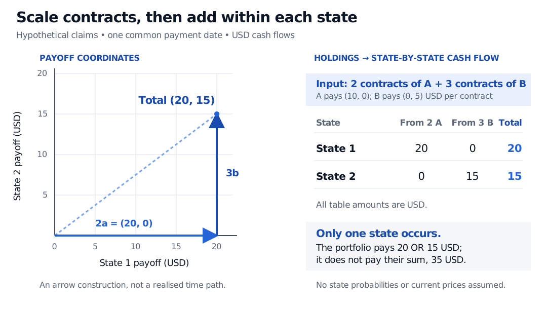
Hypothetical claims A and B pay (10, 0) and (0, 5) USD per contract across two alternative states. Two A contracts and three B contracts trace a blue tip-to-tail construction to (20, 15) USD. The ledger pays USD 20 in state 1 or USD 15 in state 2, not USD 35.
Original two-state claim example at one common payment date. The plane records alternative-state payoffs in USD; the input coefficients count contracts. Equal axis scales preserve the arrow construction. No probabilities or current prices are assumed.
Here the holding vector(2,3) is indexed by instruments and measured in contracts. The payoff vector(20,15) is indexed by states and measured in USD. They both have two entries, but describe different objects. The coefficients are neither state probabilities nor automatically portfolio weights. To obtain capital weights, one would also need the instruments' current prices and a defined investment budget.
The same calculation as a matrix product
Put the instrument payoff vectors in the columns of a matrix. Rows retain the state order:
Aq=[10005][23]=[2015].
The matrix entries are USD per contract, the inputs are contracts, and the outputs are USD. Reading a row checks one state's total; reading the columns shows the scaled instruments being combined. This is the column interpretation developed in Strang's MIT lecture.
Working backwards, a target (x,y) USD requires qA=x/10 and qB=y/5 contracts, with the denominators understood as the corresponding USD-per-contract payments. These two columns are linearly independent, so the holdings are unique. They form a basis of this two-state payoff space.
Uniqueness does not hold for every list of instruments. If a third claim C pays c=a+b, the same target can also be written a+2b+c. Adding a redundant claim creates another representation without enlarging the span, the set of all unrestricted linear combinations.
Algebra allows a short; a trading mandate might not
The combination 2a−b=(20,−5) USD is mathematically valid. Financially, it means holding two A contracts and selling one B contract short, with an obligation to pay USD 5 in state 2. A long-only mandate cannot construct this payoff from A and B: every nonnegative holding produces nonnegative state payments.
With unrestricted real holdings, these two claims span the whole payoff plane. With nonnegative holdings, they reach only its nonnegative quadrant. Integer contract rules, position limits and a budget can restrict the attainable set further. A formula that permits any real coefficient therefore describes a broader set than many desks can actually trade.
Matching a payoff is only part of valuing it
The example establishes replication in its stated two-state model. If the rows were merely a few stress scenarios rather than an exhaustive state description, matching them would establish only a scenario match.
If today's prices per contract are pA and pB, buying the illustrated holdings costs 2pA+3pB before trading costs. In a frictionless, arbitrage-free market where the target claim and its replicating portfolio can be bought and sold, identical promised cash flows and contractual terms imply equal current prices. Establishing that pricing conclusion needs those market assumptions; the vector equality alone supplies neither current prices nor a discount rate. Borrowing restrictions, bid–ask spreads, fees, margin and counterparty terms also affect an executable comparison. The Options Industry Council explains these restrictions when using synthetic portfolios in arbitrage arguments.
For more geometric examples and the passage from one combination to an entire span, see Vectors, Linear Combinations, and Span. A public preview is available; the full lesson requires membership.
Sheldon Axler, Linear Algebra Done Right, fourth edition, §2A, definitions 2.2 and 2.4, and §3C, result 3.50. The second edition treats combinations and span in Chapter 2, p. 22.
John C. Hull, Options, Futures, and Other Derivatives, ninth Global Edition (Pearson Education Limited, 2018), §§5.2, 11.2 and 11.4.
Options Industry Council, “Put/Call Parity”, “Arbitrage” and “Synthetic Relationships.”