A matrix is an ordered rectangular array. Read its shape, labels and units, then use a factor-loading ledger to map three asset weights into two exposures.
Matrix
A matrix is a rectangular array of numbers with an ordered set of rows and columns. Its shape is written m×n: m rows first, then n columns. The entry aij lies in row i, column j.
In finance, the labels are as important as the entries. A matrix might store daily returns with dates down the rows and assets across the columns, or factor loadings with factors down the rows and assets across the columns. The numbers alone do not tell you which interpretation applies.
Three assets, two factor exposures
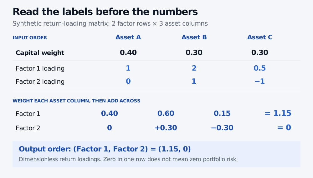
Suppose a synthetic portfolio holds assets A, B and C. Each asset's decimal return responds linearly to two factor decimal returns, plus an asset-specific residual. Hold the weights and model loadings fixed for this calculation. Put the loadings in
B=[10210.5−1].
This is a 2×3 matrix: rows are Factor 1 and Factor 2, in that order; columns are A, B and C, in that order. For example, b23=−1 means asset C's loading on Factor 2 is minus one. With other contributions held fixed, a one-percentage-point Factor 2 move contributes minus one percentage point to C's return in this model. It is a sensitivity statement, not a forecast of C's total return.
Allocate 40%, 30% and 30% of initial portfolio value to A, B and C. The vector of capital weights must use the same asset order:
The output has two entries, one per factor. The portfolio's Factor 1 loading is 1.15; its Factor 2 loading is zero. All the loadings here are dimensionless ratios of decimal returns, and the capital weights are dimensionless fractions. Different factor definitions, such as a rate measured in basis points, would require different entry units.
Synthetic matrix exposure ledger: asset weights 0.4, 0.3 and 0.3 turn factor rows 1, 2, 0.5 and 0, 1, minus 1 into portfolio loadings 1.15 and zero.
Original synthetic exposure ledger. All loadings and weights are dimensionless; each factor is measured as a decimal return. Asset and factor order are fixed.
There are two useful readings. Each row asks one question: what is the portfolio's loading on this factor? Each column contains one asset's complete two-factor profile. Scaling those columns by the capital weights and adding them is a linear combination. The matrix multiplication page develops the general calculation.
A separate cash check makes the interpretation concrete. On initial capital of USD 1,000,000, the allocations are USD 400,000, USD 300,000 and USD 300,000. A hypothetical +1 percentage-point Factor 1 shock, with Factor 2 and residual returns zero, contributes USD 4,000, USD 6,000 and USD 1,500 respectively. Total model profit is USD 11,500, or 1.15% of initial capital. The zero second loading means the stipulated Factor 2 contributions cancel; Factor 1 exposure, residual risk and model error remain.
Shape is a constraint; labels are a contract
A 2×3 matrix maps a three-entry column vector to a two-entry column vector. Reordering the asset columns requires the same reordering of the weights. A calculation can have compatible dimensions and still be economically wrong if it pairs A's loading with C's holding.
A transpose exchanges rows and columns. Thus B⊤ is 3×2, with assets as rows and factors as columns. That alternative storage convention is equally valid, but the same portfolio exposures are written as the row vector w⊤B⊤. Transposing is not a way to ignore labels.
A matrix is square when its row and column counts agree. A vector can be stored as a one-column matrix. Our loading matrix is rectangular, so it has no ordinary two-sided matrix inverse. Even a square matrix need not be invertible.
For the next step, Matrices and the Column Picture of Ax develops the two interpretations and reachable outputs. The public page is a preview; the full lesson requires membership.