Matrix transpose: Definition & Examples

The transpose of a matrix exchanges its row and column positions. If

A

has

m

rows and

n

columns, its transpose

A^\top

has

n

rows and

m

columns, with

(A^\top)_{ij}=A_{ji}.

A row becomes a column in the same order. The entries keep their values and meaning: transposing a holdings table does not buy or sell anything. It changes how those holdings are organised for a calculation.

Two desks, three assets

Suppose two desks hold three assets. Rows identify desks, columns identify assets, and each entry is a number of shares:

A=\begin{pmatrix}1&2&3\\4&5&6\end{pmatrix}, \qquad A^\top=\begin{pmatrix}1&4\\2&5\\3&6\end{pmatrix}.

A

2\times3

;

A^\top

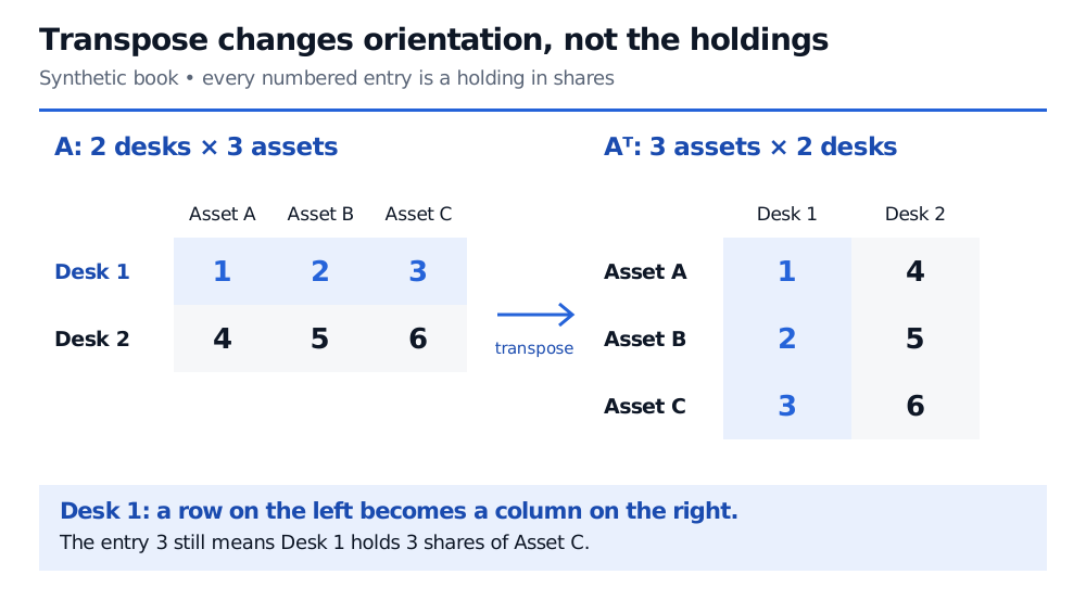
3\times2

. Desk 1's holdings

(1,2,3)

move from the first row to the first column. Asset C's holdings

(3,6)

move from the third column to the third row. The labels must travel with their rows and columns. Keeping the old labels on the transposed table would change what the data claim to represent.

Synthetic holdings in shares: the two-by-three table has Desk 1 holding 1, 2 and 3 shares of assets A, B and C, and Desk 2 holding 4, 5 and 6. Its three-by-two transpose puts assets in rows and desks in columns; Desk 1's row becomes its column without changing quantities.

Original synthetic holdings table. The highlighted row becomes the highlighted column; all six quantities and their desk–asset identities remain the same.

Now let the three assets' price changes be the column $p=(2,-1,1)^\top$ , measured in USD per share. With positions held fixed and ignoring trading costs and other cash flows, the desks' price-change P&Ls are

Ap= \begin{pmatrix}1(2)+2(-1)+3(1)\\4(2)+5(-1)+6(1)\end{pmatrix} =\begin{pmatrix}3\\9\end{pmatrix}\text{ USD}.

Transposing the result gives the row $(3,9)$ . The same row can be calculated as $p^\top A^\top$ . Transposition changes the orientation of the calculation, while preserving which shares earn which price changes.

Why a transposed product reverses order

For compatible matrix multiplication,

(AB)^\top=B^\top A^\top.

The dimensions expose the reason the reversed order is necessary:

Object	Shape
$A$	$m\times n$
$B$	$n\times k$
$AB$	$m\times k$
$(AB)^\top$	$k\times m$
$B^\top A^\top$	$(k\times n)(n\times m)=k\times m$

Simply writing $A^\top B^\top$ generally does not even give compatible inner dimensions. When square shapes happen to fit, that order is still generally wrong.

Entry by entry, the identity follows from

\begin{aligned} \bigl((AB)^\top\bigr)_{ij} &=(AB)_{ji}=\sum_{\ell=1}^n A_{j\ell}B_{\ell i},\\ (B^\top A^\top)_{ij} &=\sum_{\ell=1}^n B_{\ell i}A_{j\ell}. \end{aligned}

These are the same sums of scalar products. For the desk example, $(Ap)^\top$ is $1\times2$ , and $p^\top A^\top$ has shape $(1\times3)(3\times2)$ .

Other useful rules are $(A^\top)^\top=A$ , $(A+B)^\top=A^\top+B^\top$ for equal-shaped $A,B$ , and $(cA)^\top=cA^\top$ for a scalar $c$ .

A small symbol that changes the output

When portfolio weights

w

and asset returns

r

are both

n\times1

columns, the portfolio's weighted return is the dot product

w^\top r=\sum_{i=1}^n w_i r_i.

For beginning-of-period weights

(0.5,0.3,0.2)^\top

and matching simple returns

(0.02,-0.01,0.03)^\top

, this is

0.013

, or 1.3%. This describes a fixed initial allocation over that period, before costs and external cash flows; an arbitrary sequence of changing weights needs a dated return calculation.

The placement of the transpose also distinguishes two different products:

$w^\top w$ is $1\times1$ , the sum of squared weights. Here it is $0.38$ .
$ww^\top$ is $n\times n$ , an outer-product matrix with entry $w_iw_j$ . Here it is $3\times3$ .

Neither expression by itself is portfolio variance. That requires the assets' covariance matrix, giving the quadratic form

w^\top\Sigma w

Transposes also build covariance estimates. Let

R

contain

T>1

matching return observations in rows and

n

assets in columns. Define centred entries

X_{ti}=R_{ti}-\bar R_i

, using each asset's sample mean. The conventional sample covariance matrix is

\widehat\Sigma=\frac{1}{T-1}X^\top X.

It is $n\times n$ : asset columns are paired with asset columns. Raw $R^\top R$ is a Gram matrix of uncentred observations, not the sample covariance matrix. Both centring and the denominator matter. Meanwhile, $XX^\top$ is $T\times T$ and pairs observations, so it answers a different question even though it contains related algebraic information.

Transpose is not inverse

A transpose exists for every rectangular matrix. An ordinary matrix inverse requires a square, nonsingular matrix and undoes its linear map. Transposition does not generally undo anything: for

D=\operatorname{diag}(2,1)

D^\top=D

but

DD^\top=\operatorname{diag}(4,1)

, not the identity. Equality

Q^\top=Q^{-1}

is a special property of real orthogonal matrices.

A real symmetric matrix satisfies

A^\top=A

. For complex entries, the adjoint instead uses the conjugate transpose,

A^*=\overline A^\top

. Plain transposition never conjugates entries. For example, the scalar

i

gives

i^\top i=-1

, whereas its conjugate product is

\overline i\,i=1

; complex inner products need that conjugation.

For a fuller treatment of the entry rules and proofs, see the “The transpose” section of Matrix Algebra: Operations, Rules, and the Transpose. Its public page provides a preview; the full lesson requires membership.

Sources

Gilbert Strang, Introduction to Linear Algebra, 5th edition, Wellesley–Cambridge Press, 2016, §2.7, pp. 109–111 — transpose rules, inner and outer products, and the distinction from inversion. The financial examples and figure here are original.
MIT OpenCourseWare, Gilbert Strang: Lecture 4 transcript, pp. 2–3 — reversing factor order on transposition and the relation between transposition and inversion.

Two desks, three assets

Why a transposed product reverses order

A small symbol that changes the output

Transpose is not inverse

Sources

Related terms

Dot product

Matrix

Matrix inverse

Matrix multiplication

Quadratic form

Symmetric matrix