Matrix inverse: Definition & Examples

The matrix inverse of a square matrix

A

is the matrix

A^{-1}

that reverses its action:

A^{-1}A=AA^{-1}=I,

where

I

is the identity matrix. If

A

converts holdings into factor exposures,

A^{-1}

converts a target exposure back into the holdings that produce it. The inverse exists only when the square matrix has full rank; it is then unique.

The superscript

-1

does not mean taking the reciprocal of every entry. Matrix multiplication combines rows and columns. Undoing it generally requires a different combination of all the entries.

From an exposure target to two positions

Consider a synthetic portfolio with two instruments and two risk factors. Let $q_1,q_2$ be instrument quantities in lots. Each factor exposure is measured in its stated risk units, with fixed linear loadings:

Exposure per lot	Instrument 1	Instrument 2
Factor 1	2	1
Factor 2	1	3

Rows refer to factors; columns refer to instruments. The exposure equation is

A\mathbf q=\mathbf b, \qquad A=\begin{pmatrix}2&1\\1&3\end{pmatrix}.

Entries of

A

carry risk-units-per-lot units. Suppose the target is

\mathbf b=(5,5)^\top

: five units of each factor. Because the determinant is

2(3)-1(1)=5\ne0

A^{-1}=\frac15\begin{pmatrix}3&-1\\-1&2\end{pmatrix} =\begin{pmatrix}0.6&-0.2\\-0.2&0.4\end{pmatrix}.

Its rows refer to instruments and its columns to factors. Its entries convert the relevant factor's risk units into lots. Therefore

\mathbf q=A^{-1}\mathbf b =\begin{pmatrix}0.6(5)-0.2(5)\\-0.2(5)+0.4(5)\end{pmatrix} =\begin{pmatrix}2\\1\end{pmatrix}.

Hold two lots of instrument 1 and one lot of instrument 2. Substitution checks both targets:

2(2)+1(1)=5

and

1(2)+3(1)=5

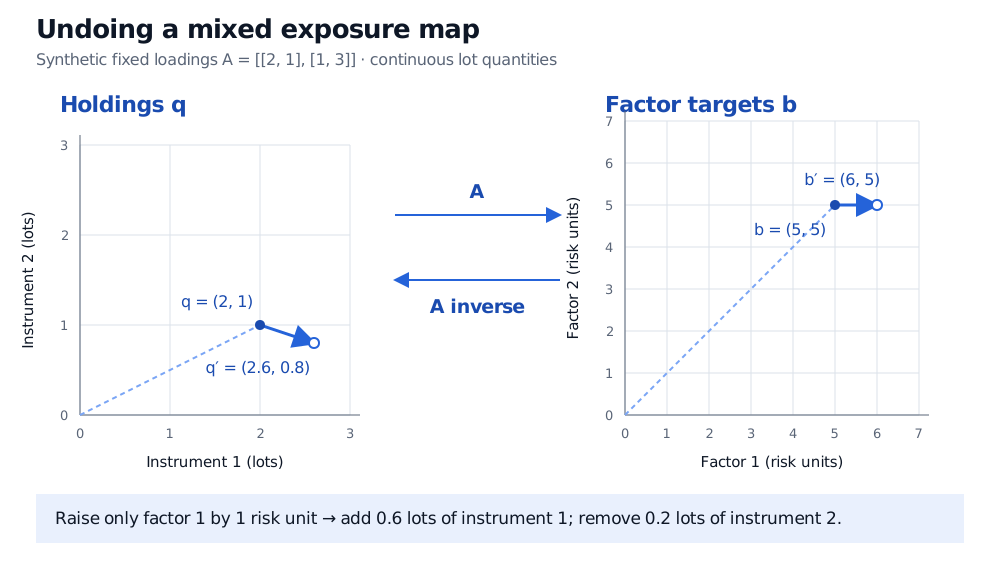
The negative inverse entries are meaningful. Each instrument contributes to both factors. To raise only factor 1 by one risk unit, the first column of

A^{-1}

says to add 0.6 lots of instrument 1 and remove 0.2 lots of instrument 2. Factor 1 rises by

2(0.6)-0.2=1

; factor 2 changes by

0.6+3(-0.2)=0

. Starting from

(2,1)

, the new holdings

(2.6,0.8)

deliver the target

(6,5)

In two separate coordinate planes, holdings of 2 and 1 lots map to factor targets of 5 and 5 risk units. Raising only factor 1 to 6 changes holdings to 2.6 and 0.8 lots. The forward arrow is labelled A and the reverse arrow A inverse.

Original synthetic fixed-loading example. The inverse isolates a target change by offsetting the instruments' overlapping exposures. Holdings axes use lots; factor axes use risk units.

This is a linear exposure model, not a statement that changing these positions generates certain profit. If loadings change with prices, time or position size, the same matrix need not describe the next rebalance.

What must be true before writing the inverse

For a square

n\times n

matrix, these conditions are equivalent: the inverse exists; the columns are linearly independent; elimination yields

n

nonzero pivots; the determinant is nonzero; and every target in

\mathbb R^n

has exactly one solution. Strang develops these relationships in §2.5 of Introduction to Linear Algebra.

A singular matrix loses information. For example,

S=\begin{pmatrix}2&4\\1&2\end{pmatrix}

has a second column twice its first. Every attainable exposure satisfies $b_1=2b_2$ . The target $(5,5)$ is impossible, while $(6,3)$ can be reached with holdings $(3,0)$ or $(1,1)$ , among infinitely many choices. No single inverse can recover a unique input from those outputs.

A rectangular matrix has no ordinary two-sided inverse. It may still have a left inverse or right inverse under appropriate rank conditions. Rectangular or rank-deficient problems can instead require least squares or a generalised inverse; their solutions need their own existence and uniqueness conditions.

Algebraic reachability also differs from trading feasibility. For the invertible matrix

A

above, target

(1,0)

has the unique unconstrained solution

(0.6,-0.2)

. A long-only desk cannot implement it. Because that solution is unique, there is no alternative long-only exact solution. Position limits, integer lots, financing and transaction costs require additional modelling.

Finding an inverse and solving a system are different jobs

For a $2\times2$ matrix, the hand calculation is

\begin{pmatrix}a&b\c&d\end{pmatrix}^{-1} =\frac{1}{ad-bc}\begin{pmatrix}d&-b\\-c&a\end{pmatrix}, \qquad ad-bc\ne0.

More generally, Gauss–Jordan elimination applies the same row operations to the augmented matrix

[A\mid I]

. If the left block becomes

I

, the right block becomes

A^{-1}

. MIT's lecture on multiplication and inverse matrices explains this construction.

For the example, the two defining checks agree:

AA^{-1}=\frac15\begin{pmatrix}5&0\\0&5\end{pmatrix}=I, \qquad A^{-1}A=\frac15\begin{pmatrix}5&0\\0&5\end{pmatrix}=I.

If the task is merely to find

\mathbf q

from

A\mathbf q=\mathbf b

, numerical software usually solves that system directly. A suitable factorisation can be reused for many targets without forming every entry of the inverse. LAPACK separates factorisation, triangular solves, condition estimation and explicit inversion into distinct operations. Choosing a direct solver avoids unnecessary work; it does not eliminate sensitivity in the underlying problem.

An existing inverse can still be dangerous to use without a conditioning check. The invertible matrix

\operatorname{diag}(1,0.0001)

has Euclidean condition number

10{,}000

. Its inverse magnifies changes in the second component by

10{,}000

. Exact invertibility alone supplies no guarantee that estimated inputs or floating-point solutions are accurate. Condition estimates, appropriate scaling and residual checks belong alongside the solve; a small residual alone cannot certify accurate holdings for an ill-conditioned system.

For a full derivation and row-reduction method, see Inverse Matrices and Gauss–Jordan Elimination. Condition Numbers develops sensitivity bounds and explains why determinant magnitude is an unreliable conditioning diagnostic. Both offer public previews; the full lessons require membership.

Sources

Gilbert Strang, Introduction to Linear Algebra, 5th edition (2016), §2.5, “Inverse Matrices”: two-sided definition, existence, uniqueness, the $2\times2$ formula and Gauss–Jordan elimination.
MIT OpenCourseWare, Gilbert Strang: Lecture 3, Multiplication and Inverse Matrices — elimination and the inverse construction.
LAPACK Users' Guide: Linear Equations — factorisation, solves, condition estimation and inversion routines.
LAPACK Users' Guide: How to Measure Errors — matrix norms, condition numbers and numerical accuracy.

From an exposure target to two positions

What must be true before writing the inverse

Finding an inverse and solving a system are different jobs

Sources

Related terms

Determinant

Identity matrix

Least squares

Linear independence

Matrix