Least squares fits a model by minimising squared residuals. Follow a return example, prove its minimum, and distinguish projection, rank, units and statistical assumptions.
Least squares
Least squares is a fitting rule: choose model parameters to minimise the sum of squared differences between observed and fitted values. In a return model, it finds the exposures whose fitted return history comes closest to the observed history under that particular loss. It does not, by itself, establish that the exposures are stable, causal or useful for forecasting.
For observations yi and model values f(xi;θ), the objective is
Q(θ)=i=1∑n[yi−f(xi;θ)]2.
A residual is the observed value minus its fitted value. Squaring prevents positive and negative misses from cancelling and makes large misses disproportionately expensive. The fitting rule can apply to a nonlinear model as well as a straight line. Ordinary least squares is the unweighted linear-model case developed here; weighted least squares assigns different weights to the squared residuals.
Which line best describes these returns?
Suppose an analyst has five aligned monthly observations of market and fund excess returns, each measured relative to the same period's risk-free return. These are synthetic teaching data. Values are quoted in percent: x=−2 means a market excess return of −2%, while differences between return quotes are measured in percentage points (pp).
Fit y^i=a+bxi. Both the intercept a and slope b are free to change. The linear regression minimises vertical misses in fund returns, treating the recorded market returns as the predictor. It does not minimise perpendicular distances on the scatter plot, and reversing the roles of fund and market defines a different problem.
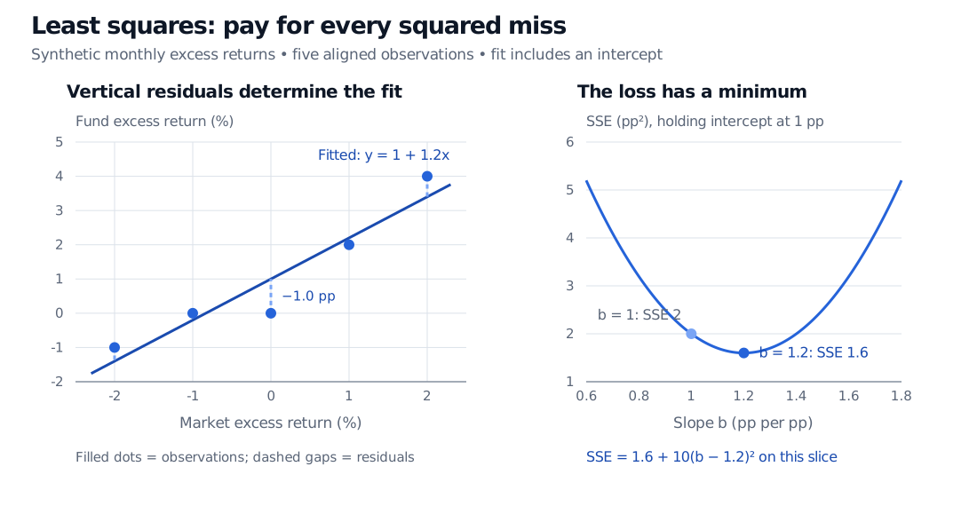
The best line is y^=1+1.2x:
Month
Market excess return x, %
Fund excess return y, %
Fitted return, %
Residual, pp
Squared residual, pp²
A
−2
−1
−1.4
0.4
0.16
B
−1
0
−0.2
0.2
0.04
C
0
0
1.0
−1.0
1.00
D
1
2
2.2
−0.2
0.04
E
2
4
3.4
0.6
0.36
The residual sum of squares, abbreviated SSE here, is 1.6 pp2. The candidate line a=1,b=1 has SSE 2 pp²; a=0,b=1 has SSE 7 pp². Neither wins. SSE is a total squared miss, not an average error, a return or a volatility.
Synthetic monthly excess-return fit: market returns −2, −1, 0, 1, 2 percent and fund returns −1, 0, 0, 2, 4 percent. The fitted line has intercept 1 pp and slope 1.2; dashed vertical residuals give SSE 1.6 pp². A second panel holds the intercept at 1 pp and shows the loss minimum at slope 1.2, versus SSE 2 at slope 1.
Original synthetic example. Filled dots show observations. The right panel is a slice of the two-parameter objective with the intercept held at 1 pp; it is not a separate fit without an intercept.
The slope says that a one-percentage-point higher market return is associated with a 1.2-percentage-point higher fitted fund return within this sample. The intercept is the fitted fund excess return at zero market excess return: 1 pp per month in this example. Five invented observations provide no evidence of persistent alpha.
If the arithmetic is new, Basic Statistics and Regression develops the mean, covariance and fitted-line formulas. The full Mathematics Primer lesson is free with a signed-in account; its public page provides a preview.
Why this is the global minimum
For a line with an intercept, provided the observed xi are not all equal,
b^=∑i(xi−xˉ)2∑i(xi−xˉ)(yi−yˉ),a^=yˉ−b^xˉ.
Here xˉ=0, yˉ=1, the denominator is 10 and the cross-product sum is 12. Hence b^=12/10=1.2 and a^=1. More decisively, expanding this particular objective gives
Q(a,b)=58+5(a−1)2+10(b−56)2.
Both added terms are nonnegative, and they vanish together only at (a,b)=(1,1.2). This proves a unique global minimum; merely comparing a few candidate lines would not.
The normal equations express the same condition in general linear-model form. Let X be the n×p design matrix, including a column of ones when an intercept is fitted, and let β contain its p coefficients. Differentiating the squared Euclidean loss gives
∇β∥y−Xβ∥22=−2X⊤(y−Xβ),X⊤Xβ^=X⊤y.
For the five observations,
X⊤X=(50010),X⊤y=(512).
Thus the fitted residual vector e=y−Xβ^ satisfies X⊤e=0: here ∑iei=0 and ∑ixiei=0. Those are fitting identities in the training sample. They do not prove that future errors will be independent of the market. Without an intercept, residuals need not sum to zero.
Geometrically, the fitted vector Xβ^ is the orthogonal projection of y onto the column space of X. The right-angle statement concerns vectors in observation space; it does not turn the vertical scatter-plot residuals into perpendicular distances to the plotted line.
The coefficients are unique exactly when X has full column rank. If every market observation instead equalled 2, only a+2b could be identified. The least-squares fitted returns would all equal the mean fund return, 1%, but infinitely many coefficient pairs would deliver that same fitted vector. In an unconstrained finite-dimensional linear least-squares problem, the fitted vector remains unique even when the coefficients do not.
Least Squares and Regression Geometry develops this projection view and its finance interpretation, with a full-membership lesson and a public preview.
What the square does—and what it cannot do
A 4 pp residual contributes 16 pp², four times the contribution of a 2 pp residual. Consequently, a small number of extreme observations can strongly affect the fit; unusual predictor values can also have high leverage. Check whether an extreme return is genuine or a data error before deciding how it should influence a financial model. Minimising ∑i∣yi−a−bxi∣ instead is a different, absolute-error or L1 fit, generally with different coefficients. Dividing the squared loss by the fixed sample size changes its scale but not its minimiser.
Units matter too. Express both series as decimal returns and the fitted intercept becomes 0.01, the slope stays 1.2, and SSE becomes 0.00016 in decimal-return-squared units. A reported SSE of 1.6 without its units is ambiguous.
Normal errors are not required to compute a least-squares minimiser. Unbiasedness, efficiency, likelihood interpretations and confidence intervals are further statistical claims. For example, a correctly specified linear conditional mean and zero conditional-mean errors support unbiasedness; the Gauss–Markov variance comparison adds a common finite error variance and no cross-observation error covariance, conditional on the design. Independent Gaussian errors with common variance connect least squares to maximum likelihood and classical exact finite-sample t and F inference, with full rank and positive residual degrees of freedom. Financial returns can violate those conditions through changing volatility, serial dependence or omitted factors.
Finally, solve the numerical problem carefully. The inverse formula (X⊤X)−1X⊤y characterises the full-column-rank solution, but explicitly forming that inverse is a poor default implementation. Forming X⊤X squares the spectral condition number for a full-column-rank design. Use a stable Householder QR decomposition, or a rank-aware method such as singular value decomposition when rank is uncertain. A stable solver can reveal a weakly identified exposure; it cannot make redundant factors informative.
Sources
Rice, John A. Mathematical Statistics and Data Analysis, 3rd ed., Duxbury, 2007. §14.1 derives the least-squares line; §14.2.1 separates its statistical properties from the minimisation rule.