Alpha measures return beyond a specified risk benchmark. Separate a realised abnormal return from a fitted intercept, raw outperformance and a forecast trading signal.
Alpha
Alpha is return beyond what a specified benchmark model attributes to a portfolio’s exposures. In performance evaluation, it usually means the intercept of a regression of portfolio excess returns on benchmark factors. A positive estimate says the chosen factors did not explain all of the sample’s average return. Establishing persistent investment skill requires more evidence.
The benchmark belongs in the definition. “The fund generated alpha” is incomplete until you know relative to which exposures, over what period, and before or after which costs. Traders also use alpha for a forecast signal, which is a different object from a measured performance intercept.
An 11% year: how much was left unexplained?
Imagine an investment committee reviewing a hypothetical fund. Over one year, the fund returned 11%, its broad equity market returned 9%, and the matched risk-free return was 3%. These are simple total returns in the same currency over the same dates. Treat the fund return as already net of investor charges for this illustration. Its market beta, supplied from a separate exposure assessment, is 1.1.
The committee first hears: “We beat the market by two percentage points.” That is correct active return: 11%−9%=2%, expressed as a return difference. But this fund carried more market exposure than the index. A zero-alpha, market-only benchmark produces
Rmodel=Rf+β(Rm−Rf)=3%+1.1(9%−3%)=9.6%.
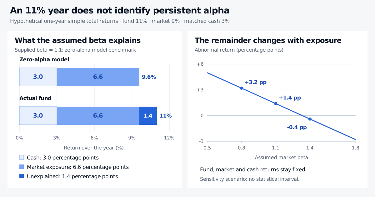
The benchmark allocates 3 percentage points to cash return and 6.6 points to market exposure. The remaining return is
ayear=Rp−Rmodel=11%−9.6%=1.4%.
This is 1.4 percentage points, or 140 basis points, of realised abnormal return relative to that model. It is smaller than the two-point index outperformance because the model attributes another 0.6 points to the fund’s extra market exposure.
Hypothetical fund return 11% consists of 3 percentage points cash, 6.6 points attributed to market exposure and 1.4 unexplained points. With returns fixed, the abnormal residual becomes 3.2 points at beta 0.8 and minus 0.4 at beta 1.4.
Original hypothetical one-year simple-return attribution. Beta is supplied separately. The right panel varies the assumed exposure, rather than showing statistical uncertainty.
One realised residual is not a statistically estimated persistent intercept. In a return-generating model with constant alpha, this year’s abnormal return contains both alpha and the year’s unexplained shock. A fortunate stock selection, an omitted exposure or an inaccurate beta can all leave a positive remainder. One observation cannot estimate an unrestricted intercept and slope together.
The CAPM itself concerns expected returns. Substituting the year’s realised market return above makes this an ex post attribution calculation, rather than a forecast of what the fund should earn next year. Nor is the 9.6% a claim that a tradable leveraged benchmark could have been implemented at the risk-free borrowing rate without costs.
The intercept behind Jensen’s alpha
For repeated observations at a fixed frequency, write portfolio and market excess returns as yt=Rp,t−Rf,t and xt=Rm,t−Rf,t. A population linear projection has the form
yt=α+βxt+εt,E[εt]=0,Cov(xt,εt)=0.
With finite second moments and positive market excess-return variance, the projection intercept satisfies
α=E[yt]−βE[xt].
Here alpha is an average component relative to the model, while εt varies across periods. It is not an assurance of positive performance every period. The population projection is a statistical description; interpreting its intercept as manager skill additionally depends on whether the benchmark captures relevant exposures and whether the return data and evaluation design are sound.
Jensen’s original paper, particularly equation (8), develops the excess-return regression and explicitly asks whether a positive observed intercept reflects ability or chance. In a sample, ordinary least squares estimates
α^=yˉ−β^xˉ.
With an intercept included, fitted residuals average to zero. The sample’s average abnormal return relative to its fitted zero-alpha benchmark is therefore α^; an individual period’s abnormal return is α^+ε^t. Keeping those two quantities separate prevents an unusually good month being mistaken for a permanent return component.
The return convention also matters. A regression of raw fund returns on raw market returns has a different intercept. If the risk-free return is constant, rearranging the excess-return equation gives a raw-return intercept of α+(1−β)Rf. A generic regression constant is not automatically Jensen’s alpha.
Report the observation frequency beside the estimate. A weekly intercept is a weekly additive regression quantity. Compounding it as though it were a certain standalone investment return does not establish an annual alpha or evidence of skill.
Change the benchmark, change the question
The figure’s sensitivity panel holds all three realised returns fixed. If the assumed beta were 0.8, the model benchmark would be 7.8%, leaving 3.2 percentage points unexplained. At beta 1.4, it would be 11.4%, leaving −0.4 points. These are alternative assumptions, not three estimates extracted from the one-year observation.
A broader performance model can account for more than market exposure:
Rp,t−Rf,t=α+k=1∑Kβkfk,t+εt.
Here the fk,t are consistently defined benchmark factor returns, such as market excess return and self-financing style-portfolio returns. Size, value, momentum, credit or liquidity exposures may matter for a particular mandate. A fund that looks exceptional against a broad equity index may look ordinary against a benchmark that captures its actual strategy. Elton and coauthors’ Chapter 26 explains why expanding the benchmark can change measured alpha.
Adding factors is not automatically an improvement. Factors should answer the economic evaluation question, use information available when required and avoid absorbing genuine decisions merely because a flexible model can fit them. Changing exposures, derivatives and nonlinear payoffs can also make a constant-beta linear benchmark misleading. Comparisons need the same model and return conventions to be meaningful.
Costs change the question again. Gross alpha asks what remains before specified charges; net alpha asks what reaches the investor after them. State which management fees, incentive fees, trading costs and financing costs are included. Deducting a flat annual fee from a published annualised regression estimate is generally an approximation unless the timing and return accounting support that calculation.
When a researcher calls a signal “alpha”
An alpha signal is an input to a trading decision: perhaps a ranking of stocks or a forecast of their next-period residual returns. A ranking score need not even have return units. Calling it alpha does not mean that a portfolio trading it has earned a positive regression intercept.
Moving from a forecast to realised net performance involves portfolio weights, risk controls, turnover, execution and capacity. The Multifactor Alpha Models lesson develops signal combination and information coefficients; its full text requires membership. That forecasting problem differs from measuring historical performance with Jensen’s regression.
What would make the claim convincing?
An estimate needs uncertainty around it. A confidence interval or intercept test must use assumptions appropriate to the errors; serial dependence and changing volatility can invalidate naive standard errors. A small p-value against zero still does not validate an omitted-risk benchmark.
Selection matters too. Picking the largest estimated alpha after screening many funds or strategy variants creates a different inference problem from evaluating one prespecified strategy. Overfitting, selective reporting and survivorship bias can inflate the apparent opportunity. Independent later data, stable definitions and feasible implementation strengthen the case for persistence.
Fama and French’s 2010 study uses bootstrap analysis to examine luck and skill across mutual funds and distinguishes returns before and after costs. Its central evaluation problem is broader than identifying a positive point estimate.
For the wider choice of performance measure, Risk-Adjusted Performance Measures compares alpha with Sharpe, Treynor and information ratios; full access requires membership. Alpha answers what the chosen model leaves unexplained. Deciding whether that remainder represents durable, investable skill requires the benchmark, data, uncertainty and implementation to withstand scrutiny.
Sources
Edwin J. Elton, Martin J. Gruber, Stephen J. Brown and William N. Goetzmann, Modern Portfolio Theory and Investment Analysis, 9th edition (2014), Chapter 26, pp. 668–669 on Jensen’s differential return and regression, and pp. 675–676 on multi-index benchmarks. All numerical examples and the figure here are original.