How fitted models and strategy searches learn noise: compare costs, preserve chronological validation and distinguish false discoveries from leakage and genuine confirmation.
Overfitting
Overfitting means adapting a model or research procedure to accidental features of the observed data, so its apparent performance overstates how well it generalises. In trading, the accident may be a few unusual returns, a favourable date range or the winning result from a large search. A simple rule selected from many alternatives can be overfit just as a large neural network can.
The practical question is whether the evidence survives outside the decisions that produced it. An attractive backtest is an observation about a research process, not a promise about future returns.
The selection rule learns too
Suppose candidate j has an unknown future performance level μj, and its development score is
μj=μj+εj.
The error εj includes sampling noise. Choosing j∗=argmaxjμj favours candidates with high true performance and favourable errors. When all candidates have the same true performance and independent, non-degenerate, mean-zero scoring errors, the expected maximum error is positive. The winning development score is then optimistic on average. The size of that optimism depends on the search and the error distribution.
This happens at two levels. A fitted model can learn noise in training observations. Separately, the researcher can overfit a validation criterion by changing features, thresholds or model families until one scores well. Cawley and Talbot's original study examines this second level: model selection itself can overfit finite-sample estimates of generalisation performance.
More flexibility creates more ways to match a sample, but flexibility alone is not a diagnosis. A complex model may capture real structure; a one-parameter rule chosen after years of searching may be heavily selected.
Twenty chances to find a false signal
Consider a deliberately simplified experiment: 20 true null hypotheses, each tested once by a valid hypothesis test with a 5% false-rejection probability. Stipulate that the rejection events are independent. Then
P(no false rejection)P(at least one false rejection)=0.9520,=1−0.9520≈0.641514=64.15%.
The expected number of false rejections is 20×0.05=1. An expectation of one does not mean exactly one appears in every experiment.
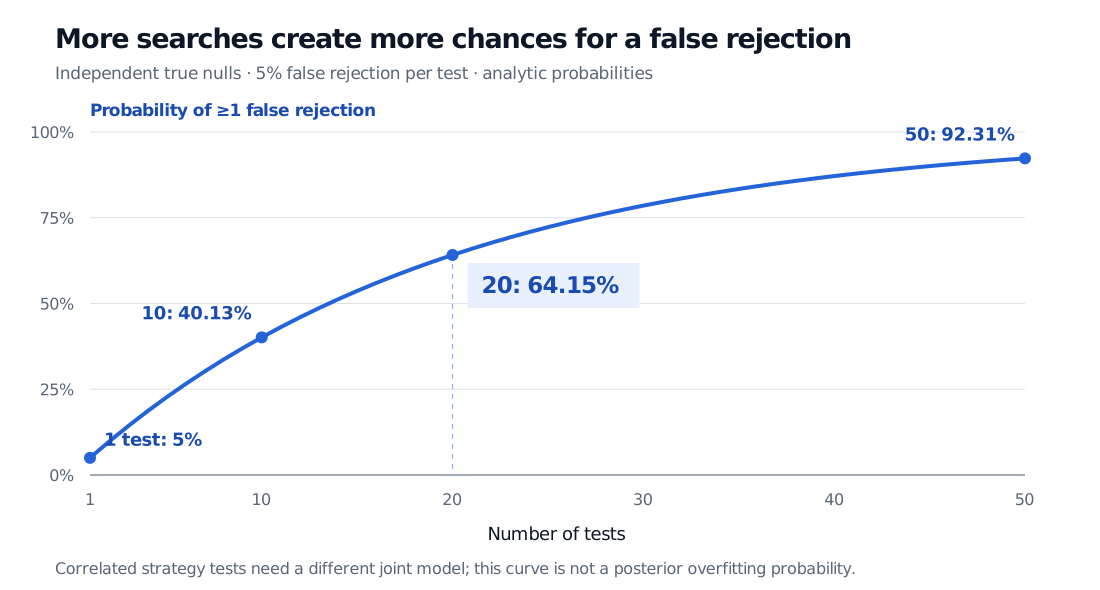
With independent true nulls and 5% false rejection per test, the probability of at least one false rejection rises from 5% for one test to 40.13% for ten, 64.15% for twenty and 92.31% for fifty.
Original analytic illustration. Independent true-null rejection events, each with probability 5%; the vertical axis is the probability of at least one false rejection, not the probability that a selected strategy is overfit.
Real strategy tests commonly share holdings, signals and market history. Their rejection events are correlated, so the independent-test formula need not apply. Nor does 64.15% give the probability that a particular strategy is false after seeing its p-value. It describes repeated experiments under the stipulated all-null model.
For a declared family of 20 valid tests, Bonferroni uses a per-test significance threshold of 0.05/20=0.0025. The probability of any false rejection is then at most 5%, without requiring independence, by the union bound. This can be conservative. It cannot repair invalid individual tests, leakage or undisclosed additional searches. Controlling false discoveries and building an economically useful strategy are different tasks.
A winner that changes when costs count
A hypothetical team investigates whether short-lived price pressure reverses after liquidity returns. That mechanism motivates a small, documented family of trading rules. It does not establish that the effect exists or can cover execution costs.
The team fits three candidate forecasting pipelines on 2018–2020 data, then compares them on the later 2021 validation period. A uses one signal, B adds a predeclared liquidity filter, and C permits several interactions and thresholds. Each candidate's preprocessing and fitted parameters use training data only. All forecasts precede the returns they predict.
Here are stipulated synthetic period averages, in basis points of the same fixed reference capital per trading day. Costs include the scenario's spread, impact, fees and financing estimates. Net equals gross minus costs; these are arithmetic P&L rates, not compounded annual returns.
Candidate
Training gross
Training costs
Training net
Validation gross
Validation costs
Validation net
A: one signal
9
6
3
8
6
2
B: liquidity filter
8
3
5
7
3
4
C: flexible interactions
32
14
18
15
14
1
C wins the training comparison and even the gross validation comparison. B wins the predeclared net validation criterion. The cost assumptions matter: the biggest gross result need not be the most useful trading result. Selecting a more flattering cost model after seeing the table would add another research choice.
The team freezes B, including its execution assumptions and update schedule, before opening the 2022 test. In this synthetic test, its gross daily average is 2 basis points and its costs average 3, giving a net average of −1 basis point per day. On fixed reference capital of USD 100,000, those means correspond to USD 20 gross, USD 30 costs and USD −10 net per day. This accounting does not assume daily compounding.
C's deterioration from training to validation is consistent with overfitting, but a performance drop alone cannot distinguish it from changing market conditions or ordinary noise. B's test loss likewise does not prove its economic mechanism is nonexistent. It does reject the tempting claim that winning validation establishes profitable implementation.
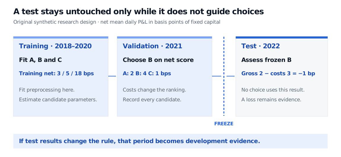
Chronological synthetic research design: training 2018–2020 fits three pipelines; validation 2021 chooses B using net average daily performance of A 2, B 4 and C 1 basis points; after a freeze boundary, untouched test 2022 evaluates B at minus 1 basis point net per day. Changing the rule after viewing the test makes that period development evidence.
Original hypothetical design. Data move forward through fitting, selection and final assessment. The freeze covers the complete procedure, including any scheduled refitting.
What protects the evidence
Overfitting, leakage and multiplicity are related, but they name different problems:
Overfitting: fitting or selecting patterns that do not generalise. It can happen with perfectly timestamped data.
Leakage: information crosses a boundary it should not cross, such as fitting a scaler on future test observations or using unavailable labels. Look-ahead bias is a temporal example. It can inflate results even with one fixed model.
Multiplicity: many opportunities to select a favourable finding. The opportunities include date ranges, universes and metrics, as well as model parameters.
Repeated holdout reuse: test results influence the next choice. That period now participates in development, even if every individual fit excludes its rows.
Use chronological development folds that match the intended learning schedule. Fit data transformations inside each eligible training window; exclude labels whose outcomes were not yet known. Where outcome intervals overlap evaluation data, remove the conflicting training samples. Randomly shuffling daily rows generally fails to reproduce this trading-information sequence.
Keep a trial register, including abandoned candidates and manual changes. Predeclare the primary metric, baseline, tuning budget and economically plausible parameter range. Regularisation or simpler models can reduce sensitivity to noise, while nested validation separates inner tuning from outer assessment. Neither technique makes an extensively reused result independent confirmation.
An untouched later test supplies useful additional evidence, with uncertainty. One period may be short, unusually favourable or unrepresentative of the future. Report subperiod behaviour, transaction costs, exposures and sensitivity to reasonable assumptions; continue with newly arriving observations and monitoring. If a failed test prompts a revised strategy, preserve that history and evaluate the revision as a new research version.
Bailey, D. H., Borwein, J. M., López de Prado, M. and Zhu, Q. J., The Probability of Backtest Overfitting, author-hosted manuscript revised February 2015, §§1–2. Research-search effects and limitations of fixed holdouts. The paper's PBO framework is distinct from the all-null false-rejection calculation above.
Hastie, T., Tibshirani, R. and Friedman, J. (2009), The Elements of Statistical Learning, 2nd ed., §7.2, pp. 219–222: model selection versus assessment and training/validation/test roles. Local grounding copy consulted.
López de Prado, M. (2018), Advances in Financial Machine Learning, §§11.2–11.6: backtest limitations, trial records and strategy selection. Local grounding copy consulted. The candidate comparison and figures here are original synthetic examples.