Backtesting: Definition & Examples

Backtesting is replaying a specified trading or investment policy on historical information to estimate the positions, cash flows and performance it would have produced under stated assumptions. A useful backtest asks whether an economic idea survives realistic timing, execution, costs and evaluation. Finding a rule that fits yesterday's price chart is only one way to produce an attractive historical result.

A trading backtest has two obligations. The simulation must account for what could have happened; the research design must explain what the result is evidence for. Correct arithmetic cannot repair future information. An untouched test period cannot repair a simulator that invents fills.

Here, backtesting means historical strategy simulation. The term also appears in risk management, where a forecast such as value at risk is compared with subsequent losses. That is a different evaluation object.

Start with a question that can fail

Suppose a researcher asks: after a stock falls, does a short-lived reversal remain profitable after paying to enter and exit? The possible mechanism is temporary selling pressure. A falsifying outcome would be that the apparent rebound occurs before a feasible entry, or is smaller than trading costs.

Before examining the evaluation period, specify the instrument universe, information cutoffs, entry and exit rules, position sizes, constraints and comparison policy. For the reversal question, an unchanged cash position is a natural initial comparison; a broader investment claim may also require a market-exposure benchmark. “We bought the stocks that subsequently rebounded” does not define an implementable rule.

The input must reflect what was available then. A financial statement's period end is not its release time; the final revised number may differ from the first published number. A historical index universe must include the names eligible at each date, including later failures. Otherwise look-ahead bias or survivorship bias can enter before any order is simulated.

Cleaning and fitting also have clocks. Estimate a normalisation, imputation rule or model using only the training information allowed at that decision. A feature with a past timestamp can still leak information if its transformation was fitted on future observations.

A four-fill backtest you can reconcile

Consider an original synthetic one-stock example. It illustrates an accounting contract, not evidence for the reversal hypothesis. Begin with USD 2,000 cash and no shares. There are no deposits, withdrawals, interest, dividends, taxes or borrowing. Each fill costs USD 1.

Freeze this rule: after a close-to-close decline of at least 1%, buy 10 shares in the next session's opening auction, then sell those shares in that session's closing auction. Remain flat otherwise. Do not short or borrow cash.

For these synthetic sessions, the opening auction is at 09:30 and the closing auction at 16:00. The final close becomes usable at 16:01. Compute the signal then, submit the next opening order at 09:25, and submit the predetermined same-session closing order at 15:45, before the assumed auction cutoff. The exit does not depend on knowing that closing price.

The five consecutive closes, from a warm-up session through Session 3, are USD 102, 100, 102, 99 and 100. The test starts after Session 0 closes; the preceding warm-up close supplies its signal. Thus the declines into Sessions 0 and 2 trigger entries in Sessions 1 and 3; the rise into Session 1 does not trigger an entry in Session 2. Stipulate sufficient auction liquidity and full fills at the following prices. These are assumed execution prices, not the best prices selected from each day's range.

Event	Filled shares	Price per share (USD)	Fee (USD)	Cash after fill (USD)	Shares after fill
Initial state	—	—	—	2,000	0
Session 1 open: buy	+10	100	1	999	10
Session 1 close: sell	−10	102	1	2,018	0
Session 3 open: buy	+10	101	1	1,007	10
Session 3 close: sell	−10	100	1	2,006	0

With signed filled quantity $\Delta q_i$ (positive for buys), fill price $p_i$ and explicit fee $f_i$ , update

q_i=q_{i-1}+\Delta q_i, \qquad C_i=C_{i-1}-\Delta q_i p_i-f_i.

Here $q_i$ is the actual holding in shares and $C_i$ is cash in USD. A signal is a forecast; a target is a desired position; an order requests a trade; a fill creates the actual holding. Only filled quantities belong in this ledger.

The two completed trades earn gross profits of USD 20 and minus USD 10. Therefore

\begin{aligned} \text{Gross profit}&=10(102-100)+10(100-101)=10,\\ \text{Total fees}&=4(1)=4,\\ \text{Net profit}&=10-4=6\text{ USD},\\ R&=\frac{2006-2000}{2000}=0.003=0.3\%. \end{aligned}

The denominator is the initial account equity, including unused cash. This is the return over the illustrated test window, not an annualised return. There is no remaining inventory to value or liquidate.

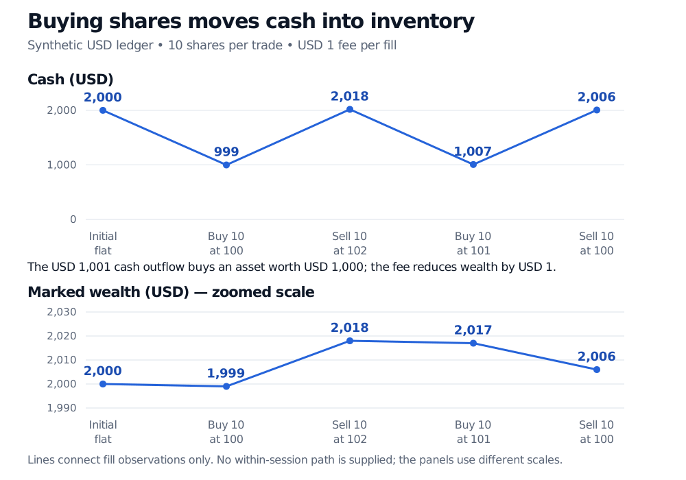
Synthetic four-fill backtest: cash is USD 2000, 999, 2018, 1007 and 2006, while wealth marked at each fill price is USD 2000, 1999, 2018, 2017 and 2006. Cash and wealth panels use different labelled scales.

Original synthetic ledger. Wealth equals cash plus shares valued at the supplied contemporaneous fill price. These are event observations with different vertical scales, not a complete intraday equity path.

The first buy spends USD 1,001 but acquires shares worth USD 1,000 at that mark. The immediate wealth loss is the USD 1 fee, not the cash spent. While inventory remains open, report marked wealth $V_i=C_i+q_i m_i$ using a declared mark $m_i$ . A mark is a valuation convention; it does not guarantee liquidation at that price.

Costs can change the trade, not just the answer

The four fills already specify execution prices. A separate transaction-cost model must say which costs those prices include. Do not subtract a spread again if it has already been incorporated into the fills. Likewise, slippage needs a named reference price and a buy/sell sign convention.

Holding these four fills fixed, fees of USD 2 per fill leave only USD 2 net profit; USD 2.50 per fill eliminates the gross USD 10 profit. That is a useful sensitivity calculation, but a larger live order can also receive worse prices, partial fills or no fill. Cash, margin and borrow constraints can change subsequent positions. Rerun the economic simulation when those states change.

Recorded daily highs and lows do not establish that an order could execute at those prices. Chan's discussion of historical data and execution in Chapter 3 makes this distinction explicit. Our auction fills remain assumptions to investigate with suitable data, rather than fills proved by the close series.

Evaluate in the order information arrives

Develop the rule and fit its parameters on earlier data. Use a later validation segment for declared selection decisions. Reserve a later test segment for evaluation of the frozen research procedure. In a walk-forward design, each refit must finish before the next evaluation window begins, using only outcomes already available then.

Chronology alone is insufficient when training outcomes extend into evaluation dates. For example, a future multi-day return used as a training label may overlap the test window. Remove the overlapping training information and apply a gap where the information structure requires it; merely sorting rows by date does not remove leakage.

Also preserve the search history. Trying many thresholds and reporting only the winner creates overfitting even when every individual ledger is accurate. Bailey and co-authors study this strategy-selection problem and explain limitations of a simple holdout. Once an evaluation result influences a revision, it has become development information; renaming it “out of sample” does not restore independence. Their analysis concerns selection uncertainty, not a substitute for causal event timing. The author-hosted paper develops that distinction.

A decision-ready report joins the reconciled net return stream to its assumptions: benchmark and exposure, maximum drawdown, concentration of gains, Sharpe ratio with its sampling limitations, cost and capacity stresses, and results by development versus evaluation period. Two trades cannot establish a stable expected return. Our sparse fill observations cannot establish the largest intervening drawdown either.

A backtest can reject a broken implementation or weaken an economic hypothesis. A promising result supports a bounded next step, such as prospective paper trading with explicit limits. It does not turn assumptions about future markets and execution into facts.

Continue with the full ledger and evaluation

Positions, Trades, Fills and P&L develops cash, holdings, partial fills and marked P&L. Backtest Evaluation connects those records to capital-flow-adjusted returns, risk and a research decision. Both have public previews; the full lessons require membership.

Sources

Ernest P. Chan, Quantitative Trading: How to Build Your Own Algorithmic Trading Business (Wiley, 2009), Chapter 3, especially the opening discussion of replication and the historical-data/execution discussion on pp. 42–43. Local grounding text inspected; the ledger and rule here are original synthetic examples.
David H. Bailey, Jonathan M. Borwein, Marcos López de Prado and Qiji Jim Zhu, The Probability of Backtest Overfitting, author-hosted revision dated February 2015, introduction and §§2.1–2.2. Supports the distinction between strategy selection and reporting one favourable simulation.

Start with a question that can fail

A four-fill backtest you can reconcile

Costs can change the trade, not just the answer

Evaluate in the order information arrives

Continue with the full ledger and evaluation

Sources

Related terms

Look-ahead bias

Maximum drawdown

Overfitting

Sharpe ratio

Slippage

Survivorship bias

Transaction cost

Value at risk