Value at risk: Definition & Examples

Value at risk (VaR) is a percentile of a portfolio's loss distribution over a specified horizon. A one-day 95% VaR of USD 3,190 means that, under the stated loss model, the probability of losing more than that threshold is at most 5%. It does not cap tomorrow's loss, and it does not give the average loss in the worst 5% of outcomes.

A useful VaR report therefore names the portfolio, currency, horizon, percentile and distributional assumptions. “VaR is 3,190” leaves too much unstated to compare two desks or decide whether an exposure fits a risk limit.

Start with a loss, then take its percentile

Use a loss-positive convention: positive numbers mean losses, while negative numbers mean gains. For a fixed long position worth

V_0

and its simple holding-period return

R

L=-V_0R.

This mapping is exact for that fixed linear exposure. An option book needs revaluation under changes in its underlying risk factors; substituting a stock-return formula can miss its nonlinear payoff.

Let $F_L(l)=\mathbb{P}(L\le l)$ be the loss cumulative distribution function. For $0<\alpha<1$ , define

\operatorname{VaR}_\alpha(L)=q_\alpha(L) =\inf\{l\in\mathbb{R}:F_L(l)\ge\alpha\}.

Read this as the first loss threshold where cumulative probability reaches the chosen level. Consequently,

\mathbb{P}\bigl(L>\operatorname{VaR}_\alpha(L)\bigr)\le 1-\alpha.

For a continuous distribution the exceedance probability is exactly

1-\alpha

. A distribution with a jump can carry cumulative probability past the target. The lower generalised inverse specifies which boundary to use; this convention is consistent with the quantile treatment in Acerbi and Tasche, definitions 2.1–2.2, after translating their profit/loss notation into positive losses and a high confidence level.

A negative VaR is possible. If a position gains USD 50 with certainty, then $L=-50$ and every percentile of that loss is minus USD 50. Replacing negative values with zero is an additional reporting policy, not this mathematical definition.

A USD 100,000 position, one day ahead

Suppose a hypothetical fixed exposure has a one-day simple return

R\sim\mathcal{N}(0.001,0.02^2),\qquad V_0=100{,}000\ \text{USD}.

The mean return is 0.1%, and its standard deviation is 2 percentage points. These are stipulated physical-return assumptions, not market estimates or risk-neutral option-pricing inputs. The dollar loss is therefore normal, with mean minus USD 100 and standard deviation USD 2,000:

\mathbb{E}[L]=-100,\qquad \operatorname{SD}(L)=2{,}000.

For normal losses with mean $\mu_L$ and standard deviation $\sigma_L$ , standardisation gives

\operatorname{VaR}_\alpha(L)=\mu_L+\sigma_L\Phi^{-1}(\alpha),

where

\Phi

is the standard normal CDF. The NIST normal-distribution reference describes the location, scale and percentile functions underlying this calculation. At 95%,

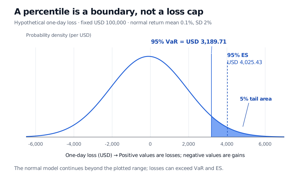
\operatorname{VaR}_{0.95}(L) =-100+2{,}000(1.6448536\ldots) \approx 3{,}189.71\ \text{USD}.

The positive mean return shifts the loss distribution left by USD 100. Using only $1.64485$ times dollar volatility would drop that mean adjustment. Raising the percentile to 99% gives USD 4,552.70 under the same model; changing the percentile changes the question even though the position is unchanged.

Hypothetical normal one-day loss has mean minus USD 100 and standard deviation USD 2,000. Its 95% VaR is USD 3,189.71, with 5% probability to the right; the average in that tail is USD 4,025.43.

Original hypothetical fixed USD 100,000 exposure: one-day simple return mean 0.1% and standard deviation 2%. The normal model extends beyond the displayed loss range.

The normal assumption makes the calculation convenient. It also assigns some probability to simple returns below minus 100%, which is incompatible with an unleveraged limited-liability asset. More generally, jumps, changing volatility and tail dependence can make this model a poor description of severe portfolio losses. A precise quantile calculation does not establish that its input distribution is adequate.

When 95% lands inside a jump

Consider a separate hypothetical loss distribution:

One-period loss (USD)	Probability	Cumulative probability
0	94%	94%
20	4%	98%
100	2%	100%

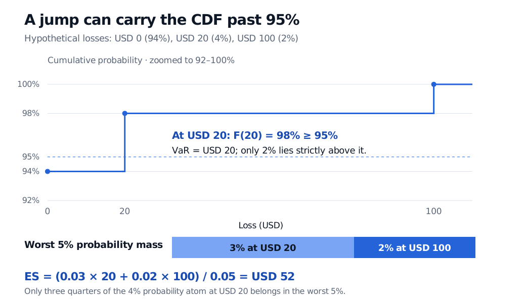
At zero the CDF has not reached 95%; at USD 20 it has. Thus 95% VaR is USD 20, although only 2% of outcomes lose strictly more than USD 20. There is no contradiction: the definition requires an exceedance probability at most 5%.

Now ask how severe the worst 5% is. Take all the 2% probability at USD 100, then another 3% probability from the USD 20 outcome. This produces expected shortfall:

\operatorname{ES}_{0.95}(L) =\frac{0.02(100)+0.03(20)}{0.05} =52\ \text{USD}.

Averaging every outcome at or above VaR gives USD 46.67: that includes 6% probability, rather than the desired 5%. Averaging only outcomes strictly above VaR gives USD 100: that includes just 2%. Fractional allocation of the probability mass at the cutoff selects exactly the required tail size. The distinction for discontinuous distributions is developed in Acerbi and Tasche, definitions 2.3–2.6 and proposition 3.2.

The loss CDF jumps from 94% to 98% at USD 20, making 95% VaR USD 20. A worst-5% allocation uses 3% probability at USD 20 and 2% at USD 100, giving ES USD 52.

Original hypothetical finite loss distribution. The CDF panel zooms to 92–100%; the allocation bar shows exactly 5% probability mass, including only three quarters of the atom at USD 20.

For the earlier continuous normal example, the worst-5% average is USD 4,025.43. VaR marks the boundary; ES uses the losses across the tail. Neither is the maximum possible loss.

Same definition, different estimation methods

Parametric VaR fits or stipulates a distribution, then inverts its CDF. The normal calculation above is one instance. Assuming normal risk-factor changes does not make a nonlinear option portfolio's loss normal.

Historical simulation applies past risk-factor changes to today's portfolio and takes a percentile of those revalued losses. It does not simply collect the desk's old profits and losses, which may reflect different positions. The historical window, weighting and treatment of changing volatility all affect the answer.

Monte Carlo VaR generates scenarios from a chosen model, revalues the portfolio and estimates the loss percentile. More draws reduce simulation noise; they do not fix a misspecified scenario model.

For

n

equally weighted losses sorted in ascending order, the empirical inverse-CDF convention gives order statistic

L_{(\lceil n\alpha\rceil)}

. Software can instead interpolate between observations. R's official quantile documentation distinguishes inverse empirical-CDF type 1 from its default interpolating type 7. Record the convention when comparing results, especially with few observations or repeated losses.

A horizon needs its own loss model

Even under normality, multiplying the whole VaR by the square root of time is not generally exact. If dollar losses are additive and iid normal, each with mean

\mu_L

and standard deviation

\sigma_L

, then their

h

-day sum has

\operatorname{VaR}^{(h)}_\alpha =h\mu_L+\sqrt{h}\,\sigma_L\Phi^{-1}(\alpha).

The mean scales with $h$ ; the standard deviation scales with $\sqrt{h}$ . For ten additive losses with the example's daily moments, 95% VaR is USD 9,402.97, versus USD 10,086.74 from multiplying its one-day VaR by $\sqrt{10}$ . Exact whole-VaR square-root scaling needs zero mean in this additive iid normal model. Compounding a buy-and-hold asset, rebalancing exposures or modelling dependent returns requires a corresponding multi-period construction.

Use VaR alongside tail severity and stress testing. A 5% forecast exceedance probability does not promise exactly five exceptions in the next hundred days. Validation should examine exception frequency, clustering, changed market conditions and what happens beyond the threshold. A VaR limit is also a policy choice: it needs a response rule and realistic execution assumptions to influence actual exposure.

Continue learning

The VaR lesson, §§2–3.1 develops the generalised inverse and normal calculation. The full lesson requires membership; its public preview provides the outline. Continue with expected shortfall to examine tail averages and cutoff mass in more detail.

Sources

McNeil, Frey and Embrechts, Quantitative Risk Management: Concepts, Techniques and Tools, revised edition (2015), §2.3.2, definition 2.8 and example 2.11; §2.3.4, definition 2.12 and lemma 2.13; §9.2.3 on historical revaluation.
Hull, Options, Futures, and Other Derivatives, 9th Global Edition, §22.1, pp. 516–519: horizon, percentile and tail-severity distinction; the exact square-root-time condition on p. 519.
Acerbi and Tasche, On the coherence of Expected Shortfall, definitions 2.1–2.6 and proposition 3.2. Their low-tail profit/loss convention is translated here to a high-percentile positive-loss convention.
NIST/SEMATECH, Normal Distribution: density, location/scale and percentile functions.
R Core, Sample Quantiles: empirical inverse and interpolating conventions.