Expected shortfall averages the worst specified fraction of losses. Calculate normal ES, allocate a discrete cutoff atom correctly, and interpret coherence without treating ES as a maximum loss.
Expected shortfall
Expected shortfall (ES) is the average loss in the worst specified fraction of a loss distribution. At 95% confidence, it averages the worst 5% of outcomes; at 99%, the worst 1%. It is also commonly called conditional value at risk (CVaR), although the word “conditional” needs care when several outcomes share the cutoff loss.
Value at risk identifies a loss threshold. ES measures the severity of the tail beyond that threshold, including just the right fraction of any probability mass at the boundary. Neither is the worst possible loss or a promise about the next trading day.
Fix the loss before averaging it
Let L be the portfolio's loss over a stated horizon, measured in a stated currency: positive values are losses and negative values are gains. The distribution might come from a model, historical scenarios or simulated portfolio revaluations. Changing the horizon, positions, valuation method or treatment of costs changes the loss being measured.
For an integrable loss, meaning E∣L∣]<∞, define the loss [quantile by
qu(L)=inf{l:P(L≤l)≥u}.
At confidence level 0<α<1, expected shortfall is
ESα(L)=1−α1∫α1qu(L)du.
This averages quantiles over the upper 1−α of probability, with equal weight per unit of probability. It does not average distinct loss amounts equally. ES has the same units as L, and it is at least as large as qα(L) under this convention. It can be negative when even the selected tail averages a gain; “risk measure” does not mean every reported number must be positive.
Integrability matters. A model with an infinite upper-tail mean can have a finite VaR while its ES is infinite. A finite simulation will still return a finite average, so a finite output alone does not establish that the model's population ES exists.
A one-day risk number for a USD 100,000 position
Suppose a hypothetical portfolio has fixed starting value USD 100,000 and one-day simple return
R∼N(0.001,0.022).
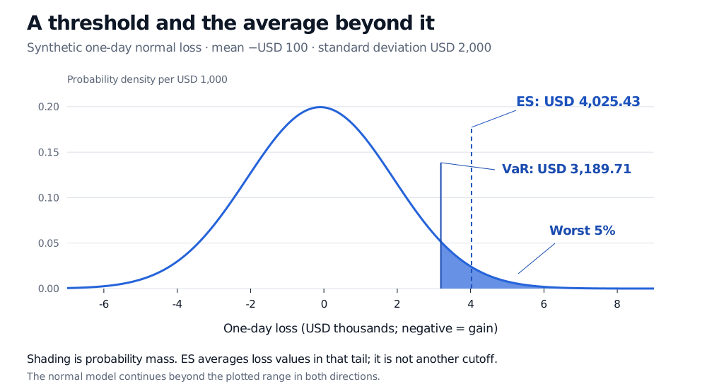
Assume that this return already describes the chosen portfolio P&L basis, with no additional cash flows. Dollar loss is L=−100,000R, so the normal loss distribution has mean μL=−100 and standard deviation σL=2,000. The negative mean loss represents an expected gain of USD 100, rather than an error in the sign convention.
Write zα=Φ−1(α), where Φ and ϕ are the standard normal distribution function and density. Then
VaRα(L)ESα(L)=μL+σLzα,=μL+σL1−αϕ(zα).
The ES expression follows by integrating losses in the normal tail: ∫z∞xϕ(x)dx=ϕ(z). At 95%, z0.95≈1.644854, giving:
One-day measure
USD
Interpretation under this model
95% VaR
3,189.71
The loss threshold with 5% probability above it
95% ES
4,025.43
The average loss within that worst 5%
Synthetic normal one-day loss with mean minus USD 100 and standard deviation USD 2,000. The rightmost 5% is shaded, beginning at VaR USD 3,189.71. Its average loss, ES, is USD 4,025.43.
Original normal-model example, with losses in USD and the horizontal axis in USD thousands. The shaded probability is 5%; its average loss is farther right than its starting threshold. The distribution continues beyond the displayed range.
The USD 4,025.43 average is neither a cap nor a forecast of the loss on every bad day. Some tail outcomes are smaller and some are much larger. Normality is a stipulated teaching model here: its unbounded simple returns even allow economically impossible returns below −100% for an unleveraged limited-liability investment. A plausible central fit does not establish a plausible extreme tail.
Why “conditional on exceeding VaR” can fail
When there is no probability mass at the cutoff q=qα(L) and P(L>q)=1−α, the familiar shorthand is valid:
ESα(L)=E[L∣L>q].
A continuous loss distribution satisfies these conditions. With an atom at the cutoff, averaging all losses strictly above it can select too little probability; including every loss equal to it can select too much. The quantile integral handles the boundary correctly. Acerbi and Tasche's original paper on coherence explains why these distinctions matter for discontinuous distributions.
Consider a separate synthetic one-day loss distribution, in USD:
Loss
Probability
Cumulative probability
0
94%
94%
20
4%
98%
100
2%
100%
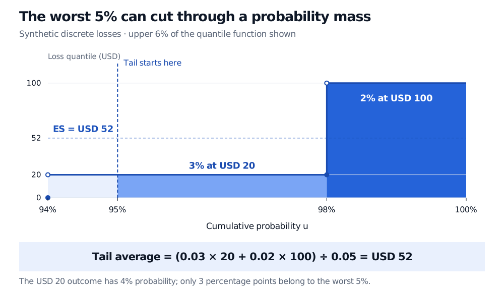
The 95% VaR is USD 20. The worst 5% consists of all 2% at USD 100, plus 3 percentage points of the 4% mass at USD 20. Thus
ES0.95=0.050.02(100)+0.03(20)=52 USD.
An equivalent mental picture is 100 equally likely scenarios: 94 losses of zero, four losses of 20, and two losses of 100. The worst five are 20,20,20,100,100, whose average is 52. No observed scenario needs to lose exactly USD 52.
Upper 6% of a synthetic discrete loss quantile function. The worst 5% begins at cumulative probability 95% and contains 3% at USD 20 and 2% at USD 100. The USD 20 atom has total probability 4%, of which three quarters is allocated to the tail. Expected shortfall is USD 52.
Original discrete example. The shaded quantile area divided by its 5% probability width gives USD 52. The plot zooms into the upper 6% of probability; the omitted 94% has loss zero.
The two tempting conditional expectations give different answers:
The first selects the worst 2%; the second selects the worst 6%. Neither selects the required 5%. Historical and Monte Carlo distributions are finite collections of scenarios, so this is a practical calculation issue even when an underlying economic model is continuous.
For a general distribution, the boundary allocation can be written explicitly:
ESα(L)=1−αE[L1{L>q}]+q((1−α)−P(L>q)).
The second term adds exactly the missing probability at q. In the example it adds 20(0.05−0.02) to the numerator. Keeping the target tail probability fixed avoids silently changing the statistic through a software quantile or tie-handling convention.
What coherence buys—and what it leaves open
On integrable losses, this quantile-based ES is a coherent risk measure: it respects loss ordering, shifts by an added certain loss, scales with nonnegative position size, and is subadditive. In particular,
ESα(L1+L2)≤ESα(L1)+ESα(L2).
Independence is unnecessary. The comparison is with the sum of standalone ES values, not with either position alone. Adding a risky position can increase total ES while still satisfying subadditivity; identical exposures can give equality. A claim that ES “always falls when portfolios are combined” misreads the inequality.
This supports consistent aggregation of desk risk limits under a common joint loss model. It does not certify that model, remove tail dependence, or account automatically for liquidation costs. Nonlinear payoffs and stressed correlations must be represented in the losses before ES can summarise them.
Estimation is another constraint. A sample of 1,000 equally weighted days allocates only 50 observations' worth of probability to a 95% tail, and ten to a 99% tail. Serial dependence, changing positions and volatility regimes reduce how much independent evidence those counts provide. Higher confidence focuses on rarer outcomes and generally raises ES under a fixed loss distribution, but leaves less data with which to estimate it. Backtesting, sensitivity analysis and stress scenarios should accompany the reported number.
Do not mechanically multiply one-day ES by a square root to obtain a longer-horizon figure. Even for iid normal additive daily losses, the mean scales with the number of days while the standard deviation scales with its square root. Rebalancing, compounding, jumps and liquidity can change the distribution further.
For the weighted-average foundations behind the discrete calculation, Expectation, Variance and Covariance works directly from probability weights. Its public page is a preview; the full lesson is available with a free signed-in account.
Sources
Alexander J. McNeil, Rüdiger Frey and Paul Embrechts, Quantitative Risk Management: Concepts, Techniques and Tools, revised edition (2015), §2.3.4, Definition 2.12, Lemma 2.13 and Example 2.14; §8.1.3, Proposition 8.13 and Theorem 8.14. These give the integrable-loss definition, normal expression, boundary correction and coherence. The scenarios and figures here are original.
Carlo Acerbi and Dirk Tasche, On the coherence of Expected Shortfall, revised manuscript dated April 19, 2002, especially Proposition 3.1, Proposition 3.2 and Corollary 4.3. Their lower-tail P&L convention is translated here into an upper-tail positive-loss convention.
John C. Hull, Options, Futures, and Other Derivatives, 9th Global Edition, §22.1, pp. 518–519, provides the continuous-tail intuition and the qualifications behind square-root horizon scaling. Its conditional-tail wording requires the cutoff qualification explained above.