The normal distribution, also called the Gaussian distribution, is a continuous probability distribution with a symmetric bell-shaped density, specified by its mean and variance. In finance it provides a tractable baseline for returns, P&L and estimation errors: a mean and volatility become probabilities of crossing a loss threshold. Those probabilities depend on the normality assumption; knowing two moments alone does not establish the shape.
Write
The expected value is , the variance is , and the standard deviation is . The second argument here is variance. A monthly return with mean and standard deviation is , not . Software interfaces may instead request a standard deviation or scale; check their parameter convention.
Read the area, not the height
The normal probability density function is
It centres the bell at ; increasing spreads the same total area of one over a wider range. Mean, median and mode coincide. These properties and the all-real-number support are summarised in NIST's distribution reference.
For any interval,
The height is a density, not . A continuous normal variable has zero probability of taking any one exact value. A density can exceed one without violating probability rules: in the monthly example, density at the mean is about 9.974 per decimal-return unit. Express returns in percentage points instead and the peak is about 0.09974 per percentage point. The density height changes with units; interval probabilities do not.
A profitable average can coexist with many losing months
Suppose a hypothetical strategy's one-month simple return, in decimal units, follows
The mean is 1% per month and the standard deviation is 4 percentage points per month. These are stipulated physical-world model inputs, not estimates from market observations or a forecast for a real strategy. All calculations below concern this one-month horizon.
To find the probability of a losing month, standardise:
Let , the standard normal cumulative distribution function. A zero return is standard deviations below the mean, so
Thus the model assigns 40.13% probability to a losing month, despite the positive mean. A positive expected return says where the distribution balances; it does not promise a positive realised return. Using or makes no difference here because exact zero has probability zero.
Now reverse the question: which return has 5% probability below it? If denotes the -quantile, then
For this model,
or −5.58%. That is a percentile of returns, not the average loss in the worst 5% of months and not a maximum possible loss. If initial wealth is USD 50,000, with fixed initial exposure and no intermediate cash flows, dollar loss is . Its 95th percentile is USD 2,789.71. This sign reversal connects the lower tail of returns to the upper tail used for value at risk.
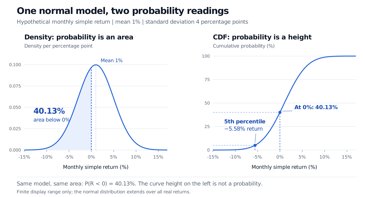
Original hypothetical monthly simple-return model, not market data. Left: probability is shaded area. Right: the cumulative curve reads the probability and inverts the 5% tail. Displayed ranges do not truncate the model.
What standardisation buys you
Every positive-variance normal distribution is a shifted, scaled version of the same standard normal. For any threshold ,
As a rough check, about 68.27%, 95.45% and 99.73% of a normal distribution lie within one, two and three standard deviations of the mean. Those are two-sided central areas. The remaining probability is split equally between the two tails; 95.45% inside two standard deviations does not mean a 4.55% probability in each tail.
An affine transformation also preserves normality:
For , the result is simply the constant . Sums of independent normal variables are normal, and portfolio linear combinations are normal when returns are jointly normal. Merely fitting each asset's marginal return to a normal curve does not establish that joint assumption. Nor does a nonlinear option payoff remain normal simply because an underlying input is normal.
For a step-by-step refresher with a different daily-loss example, the Mathematics Primer's Normal Distribution lesson is available in full with a free signed-in account; its public link opens a preview.
Where the bell curve stops helping
A normal distribution gives positive probability to every nonempty finite interval on the real line. For an unlevered long investment whose value cannot become negative, simple returns cannot fall below −100%. A nondegenerate normal simple-return model always assigns some probability below that boundary, however small it may be for a particular parameter choice. It is therefore an approximation for that investment, rather than an exact support-respecting description.
Modelling the log return as normal instead makes the gross return an exponential of a normal variable. This leads to the lognormal distribution and positive prices in geometric Brownian motion. It fixes that support problem; it does not by itself establish realistic tail behaviour.
Financial returns can exhibit heavier tails than a fitted normal distribution, asymmetry and changing volatility. A Federal Reserve Bank of Boston discussion of risk-management failures explains why extrapolating extreme-event probabilities from a bell curve can understate losses. Check tail behaviour and parameter stability against relevant data and stress scenarios; a precise CDF calculation cannot validate the model that supplied its inputs.
The central limit theorem explains normal approximations for appropriately standardised sums under conditions such as independent, identically distributed inputs with finite, positive variance. It does not make the original observations normal or guarantee an accurate far-tail approximation at a given sample size. Likewise, standardising a non-normal return produces a dimensionless score, but does not make its probabilities equal to .
Finally, the normal CDF appears in option-pricing formulas under model-specific risk-neutral probabilities. Those valuation probabilities and their drift inputs must not be read automatically as physical forecasts of how often an investment will gain or lose.
Practice
1. A dollar-loss threshold. A desk stipulates one-day P&L in USD. Find the probability of losing more than USD 1,500 and the 1st percentile of P&L. Does the latter put a floor under losses?
Answer. Losing more than USD 1,500 means , not . Standardising gives , so the probability is . The 1st percentile is . The model assigns 1% probability below that P&L; it is not a loss floor. The normal distribution has no finite lower bound.
2. A standardised surprise. A colleague observes a return two estimated standard deviations below its sample mean and reports a normal left-tail probability of about 2.28%. Does the score alone establish that probability?
Answer. No. The arithmetic gives a score of . The 2.28% figure additionally assumes an applicable normal model with suitable parameters. The score alone does not establish the distribution; parameter estimation and changing volatility can further affect the forecast. Under an exact standard normal model, .
Sources
- Dimitri P. Bertsekas and John N. Tsitsiklis, Introduction to Probability, 2nd edition (2008), §3.3, “Normal Random Variables”; §4.1, Example 4.5, for linear transformations. Local source text checked. All financial examples, practice questions and figures here are original.
- NIST/SEMATECH e-Handbook: Normal Distribution — density, support, standard form and distribution properties.
- Ralph C. Kimball, Federal Reserve Bank of Boston: Perils and Pitfalls in Risk Management, September 2000 — empirical non-normality and the danger of extrapolating rare outcomes. Historical discussion, not a statement of current capital rules.