Expected value: Definition & Examples

Expected value is a probability-weighted average of a random quantity's possible values. Also called its expectation or mean, it tells a quant the average implied by a specified probability model. It does not identify the most likely outcome, promise a profit, or say how much risk surrounds that average.

If a random variable $X$ takes values $x_i$ with probabilities $p_i$ , its expected value is

\mathbb{E}[X]=\sum_i p_i x_i, \qquad p_i\geq0,\quad\sum_i p_i=1.

The result keeps the units of $X$ : expected dollars for a dollar profit, expected orders for a count, or an expected return for a return. Percentages and the idea of assigning probabilities are enough to follow the example.

A strategy wins often and still has negative expectation

Leah is reviewing a fictional one-period trading opportunity. Her scenario model assigns these probabilities to profit or loss on a fixed position, before a known USD 20 trading cost:

Scenario	Probability	Profit or loss before cost	Contribution to expectation
Ordinary gain	70%	+400 USD	+280 USD
Moderate loss	20%	−300 USD	−60 USD
Large adverse move	10%	−2,500 USD	−250 USD

These are stipulated model probabilities, not observed market frequencies. The scenario list is assumed exhaustive and mutually exclusive. The position's gains and losses are already included; the USD 20 cost has not yet been deducted.

The model gives

\mathbb{E}[X]=0.7(400)+0.2(-300)+0.1(-2{,}500) =-30\text{ USD}.

The strategy wins in 70% of the modeled cases. Nevertheless, the relatively infrequent large loss makes its expected profit negative. Counting wins without counting their sizes would miss that result.

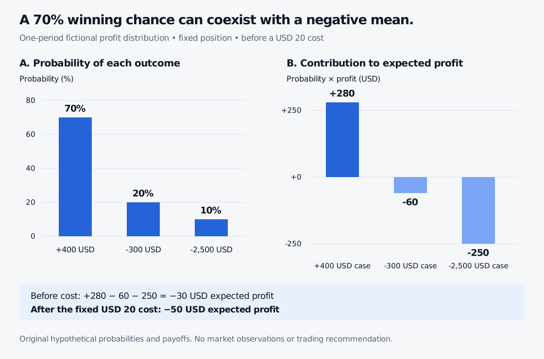
A fictional strategy has a 70 percent chance of gaining 400 USD, a 20 percent chance of losing 300 USD, and a 10 percent chance of losing 2500 USD. Their expected-value contributions are plus 280, minus 60 and minus 250 USD, totaling minus 30 USD before cost.

Original hypothetical distribution. Probabilities describe frequency within the model; probability times profit describes contribution to its mean. The graphic is not market data or a strategy backtest.

Subtract the deterministic cost once:

\mathbb{E}[X-20]=\mathbb{E}[X]-20=-50\text{ USD}.

The three net outcomes are now +380, −320 and −2,520 USD. None equals −50 USD. An expectation need not be a value that one trade can actually produce.

There is also no instruction here to make a trade whenever its expectation is positive. A decision needs the variance, adverse outcomes, funding and position constraints, and confidence in the probabilities. A small favorable mean can coexist with an unacceptable loss.

Where did the probabilities come from?

The weighted sum is easy once the distribution is specified. Establishing that distribution is usually the harder research problem.

If the 70%, 20% and 10% numbers came from historical trades, Leah would need to inspect sample size, costs, market conditions and selection bias. An outcome absent from a small sample does not necessarily have zero probability. Repeatedly selecting the best-looking backtest can also make an estimated mean overoptimistic.

A sample mean averages observations. A model expectation averages possible outcomes using their modeled probabilities. The sample mean can estimate an expectation, but they are different objects. Monte Carlo simulation similarly uses simulated observations to estimate a model's mean, with numerical sampling uncertainty in addition to any errors in the model itself.

Under suitable conditions, a law of large numbers connects repeated averages to the expectation. It does not ensure that a finite sequence is profitable, that market conditions stay fixed, or that a desk can survive until an average becomes representative.

Linearity lets you add averages without assuming independence

For random quantities with finite expectations and fixed numbers $a$ and $b$ ,

\mathbb{E}[aX+bY]=a\mathbb{E}[X]+b\mathbb{E}[Y].

No independence assumption is needed for this identity. Dependence matters when calculating the distribution or risk of the sum; it does not prevent adding its expectations. Leah's known cost is the same principle applied to a constant.

For another desk task, let $I_j$ equal 1 if order $j$ is rejected and 0 otherwise. If each of 100 orders has marginal rejection probability 2%, then

\mathbb{E}\!\left[\sum_{j=1}^{100}I_j\right] =\sum_{j=1}^{100}0.02=2.

The expected count is two even if rejections cluster during a system outage. Clustering changes risk and the probability of seeing no rejections; those require more information about dependence. Two expected rejections does not mean exactly two will occur.

SelfMadeQuant's expected-value interview examples extend this method to random counts, waiting times and stopping rules. Each problem changes which assumptions justify the calculation.

An expectation always belongs to a model

For a continuous random variable with density $f_X$ , the corresponding weighted average is

\mathbb{E}[X]=\int_{-\infty}^{\infty}x f_X(x)\,dx.

The finite-mean convention used here requires

\mathbb{E}[|X|]<\infty

. Every finite scenario table above satisfies it. Some heavy-tailed models have no finite expectation; an apparently balanced positive and negative tail is not enough to declare the mean zero. StatLect's definition and expectation properties give the fuller mathematical conditions.

The probability measure also matters in finance. A physical expected payoff describes an assumed real-world distribution. A derivative price generally needs additional valuation assumptions. In a basic constant-rate arbitrage-free option model, for example, valuation uses a discounted risk-neutral expectation, rather than simply replacing an uncertain payoff with its physical mean. The Black–Scholes explanation shows why the expected stock return disappears from that particular pricing formula.

For the mathematical foundation, Expectation, Variance and Covariance develops probability-weighted averages and the risk around them. The full primer topic is available with a free signed-in account.

References

Bertsekas and Tsitsiklis, Introduction to Probability, 2nd ed., Chapter 2 §2.4: discrete expectation, finite-mean conditions and linearity. Local grounding text; all trading numbers and illustrations here are original.
Marco Taboga, StatLect: Expected value and Properties of expected value.
OpenStax, Introductory Statistics 2e, §4.2: Mean or Expected Value and Standard Deviation, for a further introductory treatment.

A strategy wins often and still has negative expectation

Where did the probabilities come from?

Linearity lets you add averages without assuming independence

An expectation always belongs to a model

References

Related terms

Black-Scholes model

Monte Carlo simulation

Variance