Compare two profit models with the same mean but different variance, distinguish squared units from standard deviation, and calculate model and sample variance correctly.
Variance
Variance is the expected squared distance of a random quantity from its mean. It measures spread around an expected value, rather than the level of that expected value. For a profit-and-loss model, it helps distinguish a relatively stable outcome from a much wider range of gains and losses with the same average.
For a random variable X with mean μ and a finite second moment,
Var(X)=E[(X−μ)2]=E[X2]−μ2.
Squaring prevents positive and negative deviations from cancelling. It also gives larger deviations more weight. Variance is nonnegative and has squared units: if X is in USD, variance is in USD squared. Its square root, the standard deviation, returns to the original units.
The same expected profit can hide nine times the variance
Arun compares two fictional one-day profit models for positions funded with the same USD 10,000 capital. Each has two equally likely outcomes. Amounts already include the stipulated trading costs; assume no cash is added or withdrawn during the day.
Model
Lower outcome
Higher outcome
Probability of each
Expected profit
A
−50 USD
+150 USD
50%
+50 USD
B
−250 USD
+350 USD
50%
+50 USD
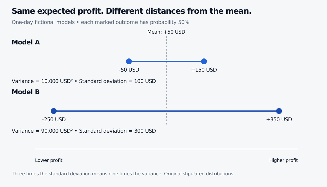
Both means are 50 USD. Model A's outcomes lie 100 USD on either side of that mean:
Var(XA)=0.5(−50−50)2+0.5(150−50)2=10,000 USD2.
Model B's outcomes lie 300 USD on either side:
Var(XB)=0.5(−250−50)2+0.5(350−50)2=90,000 USD2.
Model B has nine times the variance, although its standard deviation is only three times as large: 300 USD versus 100 USD. Comparing 90,000 USD squared with a 50 USD mean as if they shared units would have no sensible interpretation.
Two fictional equally likely profit distributions share a 50 USD mean. Model A pays minus 50 or plus 150 USD, 100 USD away from the mean. Model B pays minus 250 or plus 350 USD, 300 USD away. Their variances are 10000 and 90000 USD squared.
Original finite scenario models, not estimated market distributions. The line shows profit amounts; the marked distances are deviations from the shared mean.
Expressing these profits as returns on the same 10,000 USD capital gives both models a 0.5% expected one-day return. Their return standard deviations are 1% and 3%. Their variances in decimal-return units squared are 0.0001 and 0.0009. A change of units changes the number, not the modeled uncertainty.
Position size enters twice
If a fixed position multiplier a scales every outcome and a deterministic amount b is added,
Var(aX+b)=a2Var(X).
Doubling Model A's position doubles its standard deviation to 200 USD but quadruples its variance to 40,000 USD squared. Subtracting a certain 20 USD fee shifts its mean from 50 to 30 USD and leaves its variance at 10,000 USD squared. If the fee itself is random or scales differently with the position, it must be included in the random cash-flow model.
This scaling result assumes the profit model scales linearly. Market impact, changing liquidity or nonlinear instruments can invalidate that assumption. A larger trade need not be a scaled copy of a smaller one.
A model variance and a sample variance answer different questions
The probability weights above define complete finite models. A researcher usually starts instead with observed profits and estimates an unknown distribution's variance.
Take four illustrative daily observations: −200, 0, 100 and 100 USD. Their sample mean is zero; their squared deviations sum to 60,000 USD squared. If we treat these four observations as a finite distribution with equal weights, the variance of that empirical distribution is
460,000=15,000 USD2.
The usual sample variance for estimating an underlying population variance uses a different divisor:
s2=n−11i=1∑n(xi−xˉ)2=360,000=20,000 USD2.
For independent, identically distributed observations with finite variance, this n−1 estimator is unbiased for the underlying variance. Estimating the mean from the same sample uses one degree of freedom. The NIST measures-of-scale reference gives this sample formula and discusses how squared deviations make it sensitive to tails.
Neither divisor should be chosen just because it produces a preferred number. State whether you are describing a supplied distribution or estimating a population quantity, and check a software function's convention. With one observation, this sample variance is undefined. With clustered or changing market returns, the independent, identically distributed model also needs scrutiny.
Diversification needs the co-movement term
Variances do not generally add in the way expectations do. For two variables with finite variances,
Var(X+Y)=Var(X)+Var(Y)+2Cov(X,Y).
The covariance term measures their linear co-movement. It can increase or reduce the sum's variance. Independence is sufficient for zero covariance; zero covariance alone does not establish independence.
That distinction is central to portfolio variance and to a long–short portfolio, where the position signs affect how common moves combine. SelfMadeQuant's Expectation, Variance and Covariance lesson works through the two-asset expression. The full primer topic is available with a free signed-in account.
Spread is one part of a risk description
Variance counts upside and downside deviations symmetrically. It does not identify the worst loss, the probability of default, funding needs or the shape of the loss tail. Different distributions can have the same mean and variance while behaving very differently in extreme cases.
Variance is also a property of a specified horizon and model. Multiplying daily variance by a number of days requires conditions about return aggregation and serial co-movement; it is not a universal annualisation rule. Some heavy-tailed distributions have no finite variance at all. A finite sample calculation cannot prove those tails are harmless.
For a spread measure in the same units as the original profit, continue to standard deviation. For uncertainty in an estimated average, standard error asks a separate question; it should not be substituted for the dispersion of individual outcomes.
References
Bertsekas and Tsitsiklis, Introduction to Probability, 2nd ed., Chapter 2 §2.4 and Chapter 4 §4.2: variance, scaling and covariance. The numerical distributions here are original.