Calculate return and dollar standard deviation, see why one sigma need not contain 68% of outcomes, and distinguish individual risk from an average’s standard error.
Standard deviation
Standard deviation measures a random quantity's spread around its mean in the same units as that quantity. When variance is finite, it is the nonnegative square root of variance:
σX=E[(X−μ)2],μ=E[X].
A dollar profit has a standard deviation in dollars. A return expressed as a decimal has a standard deviation in decimal-return units. Standard deviation describes dispersion; it is not a maximum loss, a promised range or the probability of a particular outcome.
Most outcomes can sit still while the tails drive the number
Sana is checking a fictional one-day return model for a fixed position. It has three outcomes:
One-day return
Probability
−10%
5%
0%
90%
+10%
5%
The expected return is zero. Entering returns as decimals gives
Var(R)=0.05(−0.10)2+0.90(0)2+0.05(0.10)2=0.001,
so
σR=0.001≈0.0316228.
The return standard deviation is about 3.1623 percentage points, commonly quoted as 3.1623% one-day volatility. In this specified model no return actually equals +3.1623% or −3.1623%. Standard deviation summarises the distribution; it does not add possible outcomes to it.
For a fixed 50,000 USD capital base, profit is X=50,000R. Its standard deviation is approximately 1,581.14 USD. The modeled profit outcomes are −5,000, zero and +5,000 USD. Converting from returns to dollars requires the position's exposure and the assumed relationship between return and profit.
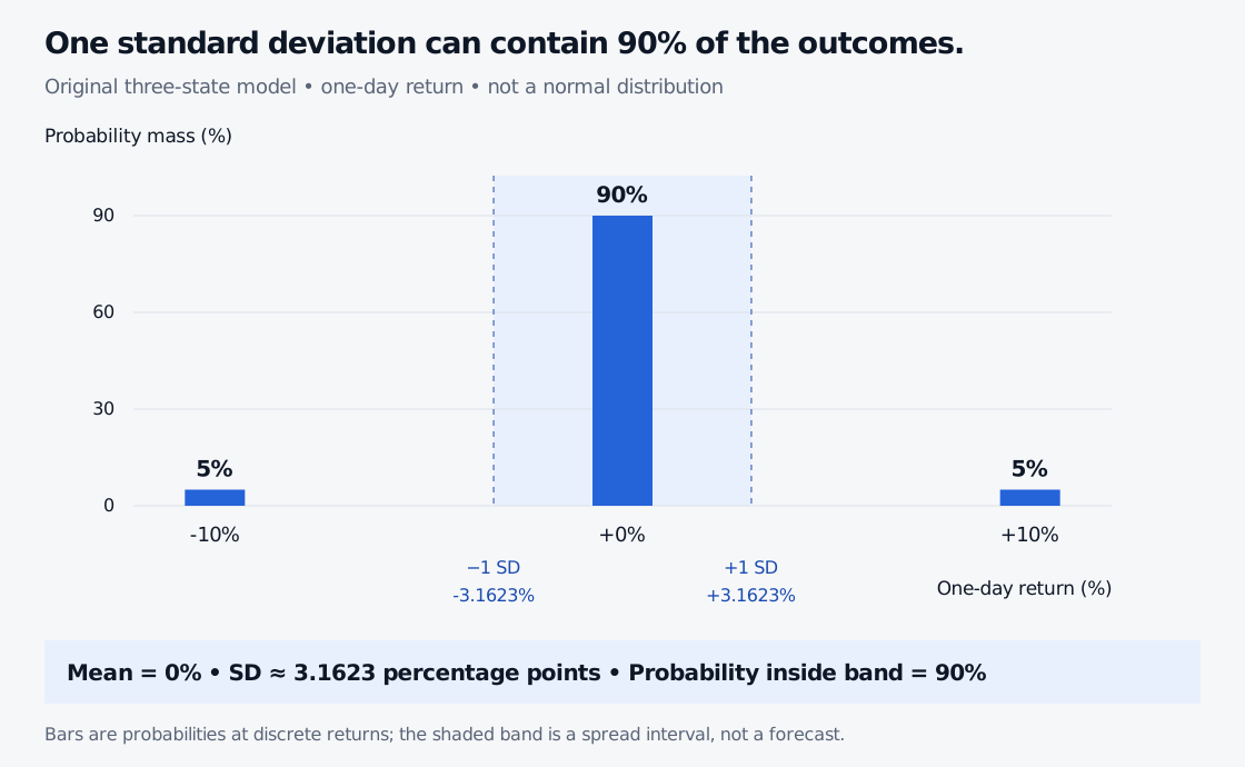
An original discrete return model assigns 5 percent probability to minus 10 percent, 90 percent to zero, and 5 percent to plus 10 percent. Its one-standard-deviation interval is approximately minus 3.1623 to plus 3.1623 percent and contains only the zero-return outcome, so it has 90 percent probability.
Original stipulated distribution, not historical data or a forecast. Vertical bars show probability mass, not density. The shaded interval extends one standard deviation either side of the zero mean.
One standard deviation does not always mean 68%
In Sana's model, the interval [μ−σ,μ+σ] contains only the zero-return outcome. Its probability is 90%, not 68%.
The familiar approximately 68.27% within one standard deviation applies to a normal distribution. It is a property of that distribution, rather than part of the definition of standard deviation. The NIST normal-distribution reference gives the underlying density and cumulative distribution.
A normal model with Sana's mean and standard deviation would be a different model: it would assign probabilities across a continuous range of returns. Matching two moments does not make the distributions interchangeable. A risk report should specify the distributional assumptions behind any tail probability.
SelfMadeQuant's Normal Distribution lesson develops standardisation and tail calculations. The full probability-and-statistics primer topic is available with a free signed-in account.
State whether the number is modeled or estimated
The three probabilities above define a complete model. With observations x1,…,xn, a common estimator is instead the sample standard deviation,
s=n−11i=1∑n(xi−xˉ)2,n≥2.
For observations −2%, 0% and +2%, the sample mean is zero and this formula gives 2 percentage points. Treating the same three values as an equally weighted finite distribution gives approximately 1.6330 percentage points, because the variance divisor is three rather than two. Those calculations answer different questions. The variance page explains the distinction and the assumptions behind the usual unbiased sample-variance estimator.
Taking a square root does not preserve unbiasedness: even where s2 is an unbiased estimator of variance, s is not generally an unbiased estimator of the population standard deviation. A larger sample can improve estimation; it does not mechanically reduce the spread of the underlying individual returns.
Standard deviation and standard error describe different spreads
Standard deviation concerns individual outcomes. The standard error of a sample mean concerns the distribution of the estimated average across repeated samples.
If 100 observations were independent draws from Sana's unchanged model, the true standard deviation of their average would be
100σR≈0.00316228,
or 0.3162 percentage points. Individual returns still have standard deviation 3.1623 percentage points. Serial dependence or a changing distribution requires a different calculation. Monte Carlo simulation provides a worked example of an estimate's error bar and its assumptions.
The same caution applies when moving between time horizons. The square-root-of-time rule requires a suitable aggregation model and assumptions about co-movement across periods. Simple returns compound multiplicatively, and correlated increments add covariance terms. Label a volatility's horizon and convention before comparing numbers.
For the basic calculation from probability weights, Expectation, Variance and Covariance is the relevant free-account lesson. For risk decisions, retain the full loss scenarios as well as this one summary number.
References
Bertsekas and Tsitsiklis, Introduction to Probability, 2nd ed., Chapters 2–3: variance, standard deviation and the normal distribution. Numerical models here are original.