Monte Carlo simulation: Definition & Examples

Monte Carlo simulation uses repeated random sampling to estimate a numerical quantity or explore a distribution of outcomes. Quants use it to value complex contracts, estimate loss probabilities and study future portfolio exposures under a chosen model.

The model specifies what can happen and with what probabilities. Monte Carlo supplies a way to calculate with that model. An expected value, for example, can be approximated by the average of simulated outcomes.

To follow the pricing example, it helps to know what an average, a standard deviation and a European call option mean. The numerical example uses hypothetical inputs, with a known analytical answer so we can inspect the simulation error directly.

A price that comes with an error bar

Leah is checking a pricing engine. A one-year call has a spot price of 100 USD and a strike of 105 USD. The model assumes 25% annual volatility, a continuously compounded risk-free rate of 4% and a continuous dividend yield of 1%.

Instead of producing one future stock forecast, the engine generates many possible terminal prices. For each one it calculates the call's payoff, $\max(S_T-105,0)$ , and discounts that payoff to today. The average discounted payoff estimates the option's model value.

There are two choices to make before drawing anything:

Calculation	Probability law used
Value this European call in the specified pricing model	The risk-neutral measure, $\mathbb{Q}$
Forecast a future profit-and-loss distribution	Typically a physical probability measure, $\mathbb{P}$ , intended to represent real-world outcomes

Risk-neutral probabilities serve the valuation calculation. They are not the desk's forecast of how often a stock will rise. For this dividend-paying stock model, the risk-neutral price drift is $r-q=3\%$ . Substituting a bullish historical return estimate would change the expectation being computed.

One random draw becomes one discounted payoff

Under risk-neutral geometric Brownian motion, terminal stock prices can be sampled directly:

S_T^{(i)}=S_0\exp\left[\left(r-q-\frac12\sigma^2\right)T+\sigma\sqrt{T}\,Z_i\right], \qquad Z_i\sim\mathcal{N}(0,1).

The $Z_i$ are independent draws from the standard normal distribution. The inputs are $S_0=100$ , $K=105$ , $r=0.04$ , $q=0.01$ , $\sigma=0.25$ and $T=1$ year. For each simulated terminal price, calculate

Y_i=e^{-rT}(S_T^{(i)}-K)^+, \qquad \widehat C_N=\frac1N\sum_{i=1}^N Y_i,

where $(x)^+=\max(x,0)$ . The target is $C=\mathbb{E}^{\mathbb{Q}}[Y]$ .

Because this contract depends only on the terminal price, one normal draw per scenario is enough. There is no daily time grid in this example. An Asian option, whose payoff depends on an average of prices, would require observations along each simulated path.

Here is the complete calculation in standard-library Python, using a fixed random seed:

from math import exp, sqrt
from random import Random
from statistics import mean, stdev

rng = Random(20261024)
s0, strike = 100.0, 105.0
r, q, sigma, maturity = 0.04, 0.01, 0.25, 1.0
n = 100_000
payoffs = []

for _ in range(n):
    z = rng.gauss(0.0, 1.0)
    terminal = s0 * exp(
        (r - q - 0.5 * sigma**2) * maturity
        + sigma * sqrt(maturity) * z
    )
    payoffs.append(exp(-r * maturity) * max(terminal - strike, 0.0))

estimate = mean(payoffs)
se = stdev(payoffs) / sqrt(n)
print(f"price={estimate:.6f}, SE={se:.6f}")
print(f"interval=[{estimate - 1.96 * se:.6f}, {estimate + 1.96 * se:.6f}]")
# price=8.889168, SE=0.050588
# interval=[8.790015, 8.988321]

The seed makes this pseudorandom experiment reproducible with this generator. It does not certify the model's assumptions or make the estimate equal to the target.

What does the reported standard error measure?

For independent, identically distributed outputs with finite variance, the estimated Monte Carlo standard error is

\widehat{\mathrm{SE}}(\widehat C_N)=\frac{s_Y}{\sqrt N}, \qquad s_Y^2=\frac{1}{N-1}\sum_{i=1}^N(Y_i-\widehat C_N)^2.

Use the standard deviation of the discounted payoffs here. The spread of terminal stock prices is a different quantity.

The law of large numbers explains convergence of the average to its model expectation. The central limit theorem supports the large-sample, approximate 95% confidence interval

\widehat C_N\pm1.96\,\frac{s_Y}{\sqrt N}.

This is an interval procedure for simulation uncertainty around a fixed model value. If we repeated independent runs at a fixed sample size, approximately 95% of the resulting intervals would cover that value when the normal approximation is adequate. It is not a 95% probability forecast for the stock, and the formula is not automatically reliable for sparse rare-event samples, dependent draws or infinite-variance outputs.

The mean formula also needs adjustment for other targets. A simulated value-at-risk is a quantile, not a sample mean; its standard error is not obtained by dividing the payoff standard deviation by

\sqrt N

This particular 95% interval misses the known answer

For Leah's assumptions, the Black–Scholes model gives a call value of 9.031036 USD. Independent deterministic integration of the discounted payoff confirms the same benchmark.

The simulation's interval, [8.790015, 8.988321] USD, does not contain it. That is possible for a 95% procedure. The example keeps its original date-based seed so the miss remains visible.

Independent scenarios $N$	Estimated price, USD	Estimated standard error, USD
1,000	8.246376	0.472524
4,000	8.822456	0.247982
10,000	8.750931	0.158317
100,000	8.889168	0.050588

The 10,000-scenario estimate is farther from the benchmark than the 4,000-scenario estimate, even though its standard error is lower. Standard error describes the scale of repeated-run variation; it is not the realised absolute error of a particular run.

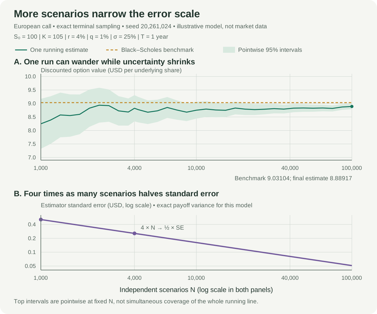
Two-panel convergence graph for a seeded European-call simulation. The upper panel shows a running estimate and approximate pointwise 95% intervals from 1,000 to 100,000 scenarios against the Black–Scholes benchmark of 9.03104 USD. The final interval misses the benchmark. The lower panel shows standard error falling in proportion to one over the square root of the scenario count.

Original simulation, seed 20261024. The upper intervals use the sample standard deviation at each checkpoint. They are pointwise intervals, not a simultaneous confidence band for the whole running curve. The lower panel uses the known payoff variance of this test model to display the exact standard-error scale.

At a fixed payoff variance, quadrupling $N$ halves standard error; reducing it tenfold requires 100 times as many samples. The same random stream supplies the successive estimates above, so those checkpoints are correlated. Repeatedly inspecting the intervals and stopping when they look favourable does not preserve the fixed-sample coverage claim.

More scenarios cannot repair every error

This example samples the exact terminal distribution of its chosen model, so there is no time-discretisation bias. A simulator that approximates an SDE on a coarse grid can instead converge very precisely to the wrong discretised expectation. More paths reduce sampling noise; finer or better time-stepping addresses that numerical bias. A continuously monitored barrier can also be missed between simulated dates.

Model risk remains even with exact sampling. Constant-volatility GBM may be a poor description of a real instrument, and estimated parameters carry their own uncertainty. Neither problem is covered by the simple Monte Carlo error bar.

Variance reduction can lower computational cost. Antithetic variates and control variates change how the estimator is constructed so less randomness survives into its output. Error estimates must then match that construction—for example, independent antithetic pair averages, rather than treating both members of each dependent pair as independent observations.

A European call is a useful test because its analytical price is available. In practice, closed-form valuation is cheaper for this example. Simulation earns its place when payoff structure, path dependence or many risk factors make other approaches difficult. Its square-root sampling rate has no explicit dimension exponent, but the cost per scenario and the payoff variance can both grow with the problem.

Calculate the benchmark and build the underlying skills

The free public SelfMadeQuant options-pricing tool computes European Black–Scholes values across spot and volatility, with rate and dividend-yield inputs. Match the example's inputs to inspect the analytical benchmark. The tool's payoff view distinguishes value today from exercise payoff; it does not run this Monte Carlo experiment.

If expectation and variance are new, start with Expectation, Variance and Covariance, part of the Mathematics Primer, available with a free signed-in account.

For the next step, Simulation and Resampling, in Probability, Statistics and Financial Data, develops Monte Carlo error estimates and distinguishes model simulation from bootstrapping observed returns. Membership is required for that lesson.

For free external study, Mike Giles' Monte Carlo lectures and example code cover sampling, error estimates, control variates and numerical path simulation. The pricing story, seed and numerical results on this page are original.

Sources

Paul Glasserman (2004), Monte Carlo Methods in Financial Engineering, Chapter 1, especially §§1.1–1.2: sampling averages, error, efficiency and risk-neutral pricing.
Mike Giles, Monte Carlo Methods, Lecture 1: GBM sampling, Monte Carlo error and variance reduction.
Mike Giles, Monte Carlo Methods, Lecture 2: Greeks, path simulation and discretisation effects.