Understand Black-Scholes assumptions, replication and risk-neutral pricing through an original European call-and-put example with dividends and a pricing-distribution graph.
The Black-Scholes model, also called the Black-Scholes-Merton model, is a mathematical model that prices options by combining an assumed stock-price process with the cost of a continuously adjusted hedge. In its standard form, the stock follows geometric Brownian motion, volatility is constant, and trading and financing are frictionless.
Its best-known result is a closed-form price for a European call or put. The deeper idea is replication: a suitable stock-and-cash strategy can reproduce the option's payoff. Under the model's assumptions, no-arbitrage pricing makes the option worth the cost of that strategy.
The model is a benchmark for valuation, hedging and quoting implied volatility. It is not a forecast of the stock price, and its price is not a promise that a real trading strategy will hedge perfectly.
The assumptions behind the number
For the dividend-paying version used here, the assumptions are:
The stock price is positive and moves continuously, with normally distributed log returns over fixed intervals. There are no price jumps.
The annual volatility σ is known and constant. It is the standard deviation scale of log returns, not a limit on the size of a move.
The financing interest rater and dividend yield q are known and constant. Both use continuous compounding. A stock holder receives dividends at the continuous rate qStdt; the option holder does not receive those dividends directly.
Traders can rebalance continuously, hold fractional shares, sell short, and borrow or lend at the same rate. There are no transaction costs, taxes or trading constraints.
The call or put in the closed-form example has European exercise: exercise happens only at its stated expiry.
The mathematical stock model under the risk-neutral measureQ is
StdSt=(r−q)dt+σdWtQ.
Here St is the stock price, t is time in years, and WtQ is Brownian motion under the pricing measure. The stock's price drift is r−q because its total return includes the dividend yield q. Under this measure the expected total return is r.
These dynamics produce a lognormal distribution for the stock price at expiry. “Lognormal” applies to the price; the corresponding log return is normally distributed. The model does not allow the stock to become negative or jump abruptly to a new level.
Pricing one dividend-paying contract
Nina needs a benchmark for two hypothetical options on a stock: one call and one put with the same strike and expiry. Each option covers one underlying unit. Both have European exercise.
Input
Value and convention
Current stock price S0
USD 120
Strike price K
USD 125
Time remaining T
180 days, using T=180/365≈0.493151 years
Annual volatility σ
25%, entered as 0.25 in the formula
Financing rate r
4% per year, continuously compounded
Dividend yield q
1.5% per year, paid continuously in the model
The 1.5% input is a proportional dividend stream, not a specified USD 1.50 cash dividend on a particular date. A stock with discrete cash dividends needs appropriate dividend treatment rather than an unexplained substitution.
For this contract, the model's call and put values are
where N is the standard normal cumulative distribution function, and
d1=σTln(S0/K)+(r−q+σ2/2)T,d2=d1−σT.
Substituting Nina's inputs gives d1≈−0.07452, d2≈−0.25008, N(d1)≈0.47030 and N(d2)≈0.40126. The prices are
C≈USD 6.84,P≈USD 10.28
per underlying unit. The exact model values before rounding are about 6.841827 and 10.284630. These are premiums today, not terminal payoffs or trading profits. A contract covering more units scales the premium by its specified multiplier.
A useful check is put-call parity:
C−P=S0e−qT−Ke−rT≈−USD 3.442803.
The separately calculated call and put agree with that identity. If one calculation silently used no dividends, or used an annual effective rate where the formula expects a continuous rate, the comparison would fail.
The Black-Scholes formula page develops the calculation further. The Black-Scholes equation describes the valuation relation from which prices can be obtained. The model is the set of dynamics and trading assumptions behind those results.
Why the expected stock return disappears
Suppose two analysts use the same spot price, volatility, rates, dividends and contract terms. One forecasts a 6% expected total stock return; the other forecasts 12%. Their Black-Scholes option price is the same. Their forecast of the stock's real-world outcome is different.
The reason is the hedge. An option and its underlying stock are driven by the same Brownian shock in this model. Holding an appropriate number of shares against the option offsets that instantaneous random exposure. The relevant share holding is its delta, and continuously updating it is delta hedging. The remaining cash position earns or pays the financing rate. The expected stock return cancels from this replication calculation.
In Nina's example, the call delta is approximately 0.466834. To hedge a short call locally, the stock component is about 0.466834 units per option unit. That is the starting hedge ratio, not a fixed position that can be left untouched until expiry. Cash financing, dividend receipts and later rebalancing are all part of the strategy.
Risk-neutral valuation gives the same price by discounting the expected payoff under Q. It uses a pricing distribution consistent with the stock's carry, rather than either analyst's physical probability measure.
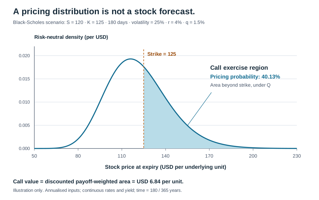
Black-Scholes risk-neutral terminal stock-price density for the worked example. The shaded area above strike 125 is 40.13% under the pricing measure, and the discounted call value is USD 6.84 per underlying unit.
Theoretical illustration, not market observations or a forecast. The stock price is lognormal under the pricing measure. The shaded area is the risk-neutral probability of finishing above the strike; the call price also weights each such outcome by the size of its payoff and discounts it.
For this call, N(d2)≈40.13% is the risk-neutral probability of finishing above USD 125. It is neither a forecast probability nor the delta, which is about 46.68%. Price, probability and hedge ratio answer different questions.
Expected stock returns still matter for investment decisions and real-world profit-and-loss forecasts. Their absence from the replication price is a conditional result of this model, not a statement that expected returns never matter in finance.
What changes outside the model
A volatility smile cannot come from one constant volatility. Real option quotes can imply different volatilities across strikes and maturities, producing a volatility smile, skew or surface. Black-Scholes remains useful as the conversion between a price and an implied-volatility quote. Fitting a separate volatility to every contract does not make those prices one constant-volatility model.
A jump cannot be hedged away by an infinitesimal stock adjustment. Jump risk, changing volatility and finite rebalancing intervals create hedging error. Bid-ask spreads, funding differences and trading costs also affect a real hedge. Local volatility and stochastic volatility models address different parts of the dynamics; the Heston model is one stochastic-volatility example. A more elaborate model still needs its assumptions checked against its intended use.
Early exercise changes the contract. The European formula does not include an American option's right to exercise before expiry. Early exercise can matter for puts and dividends. The same Black-Scholes stock dynamics can be used in an American-option valuation problem, but the exercise decision requires an additional solution step. Calling the European formula an American price is a contract error, not a small rounding approximation.
Try the benchmark, then study the hedge
Open SelfMadeQuant's free public Options Pricing tool. Enter spot 120, strike 125, 180 days, volatility 25%, risk-free rate 4%, dividend yield 1.5%. Select call and then put to reproduce the rounded values above. The tool uses a 365-day year, continuously compounded rate and yield, and annual volatility.
Its heatmap varies spot and volatility; its curves compare model value today with payoff at expiry. The expiry payoff excludes the premium. The tool implements European Black-Scholes scenarios; it does not price early exercise or discrete cash dividends.
If the contract language is new, start with the Options primer lesson, available in full with a free signed-in account. For the replication argument and formula derivation, continue to The Black-Scholes PDE, Formula and Implied Volatility, whose public page is a preview and whose full lesson requires membership. The continuous-dividend derivation explains the dividend cash flow in the hedge; its full lesson also requires membership.
The example uses the European dividend-yield formulas in John C. Hull, Options, Futures, and Other Derivatives, 9th edition, Global Edition, Chapters 15 and 17. MathWorks' Black-Scholes pricing reference independently documents the European exercise and continuous-rate/yield input conventions. All numerical inputs and the figure here are original teaching scenarios.