IV is a model-based way of expressing an option price. It is not a direct measurement of future realised volatility, or a probability that the stock will move by a particular percentage.
The example below assumes you know what a call option, its premium and its strike mean. The exercise right is important: the contract here is European.
The dealer quotes a price; the desk wants a volatility
| Input | Value and convention |
|---|---|
| Spot | 100 USD |
| Strike | 105 USD |
| Time | 1 year; equivalent to 365 days on an Actual/365 fixed basis |
| Financing rate | 4% per year, continuously compounded |
| Dividend yield | 1% per year, paid continuously in the model |
| Exercise | European call, exercise only at expiry |
| Fictional bid / midpoint / ask | 9.10 / 9.20 / 9.30 USD |
Arun holds those inputs fixed and varies only volatility. The BSM call formula is
where is the standard normal cumulative distribution function. Trial values give:
| Annual volatility input | Model call price, USD |
|---|---|
| 20% | 7.057139 |
| 25% | 9.031036 |
| 30% | 11.001092 |
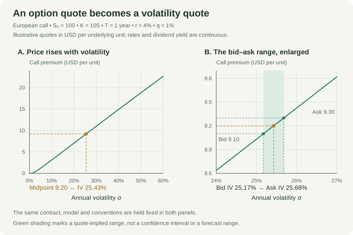
The quoted midpoint, 9.20, lies between the prices at 25% and 30%. Solving more precisely gives
Why there is one answer—and when there is none
For positive spot, strike, remaining time and volatility, BSM call vega is positive:
where is the standard normal density. The call-price curve therefore increases with volatility. Its endpoint limits are
Here and USD. For :
| Quoted price | Inversion result under these model assumptions |
|---|---|
| Strictly between and | One finite, positive implied volatility |
| Exactly | The zero-volatility limit |
| Exactly | Approached as volatility tends to infinity; no finite IV |
| Outside those bounds | No compatible BSM volatility |
At expiry, , the option value is its terminal payoff regardless of volatility. A matching price therefore cannot identify IV at all. A finite solver search limit is another distinct issue: failing to bracket a valid root below an arbitrary cap does not prove that no mathematical root exists.
A reliable search keeps the price bracket
Define . The prices at 20% and 30% give opposite signs, so the root lies between them. The bisection method repeatedly halves that interval, keeping the half that still brackets the quote. A numerical implementation should check both the remaining volatility interval and the price residual.
Newton–Raphson can converge much faster near the solution:
Its denominator explains the difficulty. When vega is tiny, a modest price discrepancy can produce an enormous or negative proposed volatility step. Deep in- or out-of-the-money options and very short maturities can be numerically delicate. A safeguarded solver can retain a valid bracket and replace an unsuitable Newton step with bisection.
Price evaluation also matters near the boundaries. Subtracting nearly equal terms or treating a rounded, almost-zero premium as exact can destroy useful information before the root search starts. A small solver residual certifies that a number fits the supplied inputs; it does not certify those inputs.
Ten cents of price uncertainty becomes volatility uncertainty
Inverting the fictional bid–ask spread gives:
| Quote | Price, USD | Annual BSM implied volatility |
|---|---|---|
| Bid | 9.10 | 25.174827% |
| Midpoint | 9.20 | 25.428355% |
| Ask | 9.30 | 25.681910% |
Locally, price uncertainty propagates as
This is a quote-implied range, not a confidence interval for some hidden “true volatility.” A midpoint is a quoting choice, and a last-traded price can be stale relative to the spot and rates used for inversion.
Keep the model and contract attached to the number
A volatility quote should travel with its conventions:
- Exercise and cash flows: a European formula omits an American option's early-exercise right. A continuous dividend yield also differs from a schedule of discrete cash dividends.
- Time and carry: use consistent expiry time, day-count convention, financing rates and dividend assumptions. Their errors can be absorbed into the inferred volatility.
- Price units: a premium per underlying unit and a premium for an entire contract must be reconciled before inversion.
- Quoting model: a futures option may use the Black model; a Bachelier model uses normal volatility with different units. Such quotes cannot be treated as interchangeable BSM percentages.
IV reflects prices for future-contingent payoffs, which is why it is often called forward-looking. It still need not equal volatility subsequently realised under real-world outcomes. Risk premia, the priced shape of tail outcomes and trading conditions affect the premium being inverted. Historical volatility, by comparison, is estimated from a chosen sample of past returns.
Repeating the inversion across strikes at one expiry produces a volatility smile or skew. Adding maturities gives a volatility surface. Different IVs across strikes show that one constant BSM volatility does not fit all those quotes; converting each price separately does not establish a single consistent stochastic model or an arbitrage-free surface.
Explore the price direction, then the shape of IV
Sources
- John C. Hull, Options, Futures, and Other Derivatives, §15.11: implied volatility and iterative inversion of option prices.
- Rüdiger U. Seydel, Tools for Computational Finance, Exercise 1.19: implied volatility as a root and stopping criteria for iterative solvers.
- J. Robert Buchanan, Solving the Black-Scholes Equation, slides 67–70: a worked implied-volatility inversion.
- The Options Industry Council, Volatility & the Greeks: vega sensitivity and its percentage-point convention.