A worked long–short portfolio example with gross and net exposure, borrow costs, beta hedging, correlation risk and a clear return denominator.
A long–short portfolio owns some assets and takes short positions in others. The long positions gain when their prices rise; the short positions gain when their prices fall. Combining the two lets a trader express a view about relative performance, adjust market exposure, or hedge an existing position. A long–short portfolio can still lose on both sides.
In equity investing, this is often called a long–short equity strategy. The portfolio structure describes the positions. It does not specify the stock-selection signal, guarantee market neutrality, or create an edge by itself.
You only need percentages and the idea of a short sale to follow the first example. Market beta becomes useful when we ask what has actually been hedged.
A good view can make money even when both stocks rise
Mira has USD 100,000 of account equity. She expects Company A to outperform Company B over the next month, but she has less conviction about the direction of the whole market.
She buys USD 100,000 of A and sells short USD 100,000 of B. For a short sale, she borrows B shares and sells them, with an obligation to return the shares later. The sale proceeds come with that liability; they are not an extra USD 100,000 of wealth. Brokerage collateral and borrowing arrangements constrain how those proceeds can be used. The SEC's introduction to short sales explains those mechanics and why a rising shorted stock creates losses.
At entry, a simplified balance sheet is:
Item
Value in USD
A shares owned
100,000
Cash, including the short-sale proceeds
100,000
Obligation to return B shares
−100,000
Account equity
100,000
This accounting example assumes no additional collateral beyond the stated equity and cash, no interest on cash or short collateral, no dividends, and sufficient margin capacity. Those assumptions make the arithmetic readable; actual brokerage terms must be modelled separately.
During the month, A rises 8% and B rises 4%.
A contributes a gain of USD 8,000.
The short B position loses USD 4,000 because replacing the borrowed shares now costs more.
The combined price gain is USD 4,000.
Both companies rose. Mira made money because the long rose more than the short.
Writing L and S for the positive initial dollar magnitudes of the long and short positions, the price-only profit and loss is
Πprice=LRL−SRS.
Here RL and RS are the assets' own price returns, not the returns of the signed positions. The minus sign accounts for the short.
For this example,
Πprice=100,000(0.08)−100,000(0.04)=USD 4,000.
The same starting positions also make USD 4,000 before costs if A falls 6% and B falls 10%. Relative performance matters; it does not require a rising market.
Costs can reverse the result
Suppose the stock borrow fee is quoted at 3% per year. For this toy month, apply a simple one-twelfth-year charge to the initial USD 100,000 short notional. The fee is USD 250. Assume another USD 200 in total entry-and-exit trading costs across the two positions.
The denominator is Mira's initial account equity. Dividing by the zero net position value would be meaningless. Dividing by USD 200,000 of gross positions would answer a different question: profit per unit of gross exposure.
A real implementation must also account for interest on eligible cash, financing charges, any short-collateral rebate, dividends received and dividend compensation paid. Borrow charges can change and may use daily marked collateral rather than this example's fixed notional. Keep those cash flows separate before combining them into a total return.
Here are three outcomes under the same simplified USD 450 cost assumption:
A's price return
B's price return
Price P&L
Net P&L
+8%
+4%
USD 4,000
USD 3,550
−6%
−10%
USD 4,000
USD 3,550
−4%
+8%
−USD 12,000
−USD 12,450
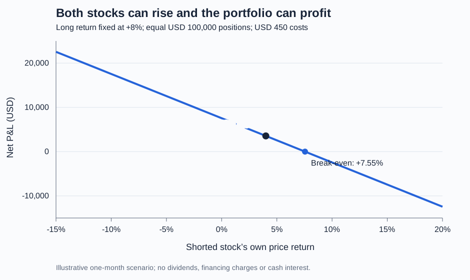
Net P&L declines as the shorted stock's return rises, with the long stock fixed at an 8 percent gain. A 4 percent short-stock gain produces USD 3,550 net profit; break-even occurs at 7.55 percent.
One-month scenario, not market data. Long and short start at USD 100,000 each; the long gains 8%; total assumed borrow and trading costs are USD 450. The shorted stock can rise substantially more than the displayed range.
Zero net exposure is not zero risk
Gross exposure measures the size of both sides. Net exposure subtracts the short side from the long side. Expressed relative to equity E,
Gross exposure=EL+S,Net exposure=EL−S.
Mira's book has 200% gross exposure and 0% net exposure. It is dollar-neutral. It is still exposed to company-specific shocks, different sector moves, changing relationships, costs and funding demands.
Even broad-market exposure need not cancel. Suppose the long stock has estimated beta 1.3 and the short stock has beta 0.8. The equity-normalised market exposure is
βportfolio=ELβL−ESβS=1.3−0.8=0.5.
Under that linear factor approximation, a 10% market rise contributes about 5% of initial equity before residual returns and costs. Equal dollar positions did not make this a zero-beta book.
To target beta neutrality with these estimated betas, Mira would need
S=LβSβL=100,0000.81.3=USD 162,500.
That changes gross exposure to 262.5% and net exposure to −62.5%, using the same initial-equity denominator. It also changes funding and margin needs. Beta neutrality is a constraint on an estimated model exposure, not a promise that a crash cannot hurt. Betas change, omitted factors matter, and forced trading can dominate the intended hedge. AQR's alternative-investing glossary distinguishes general long–short equity from strategies explicitly designed to be market neutral.
Correlation changes the risk of the spread
With positive long and short weight magnitudes wL=L/E and wS=S/E, the variance of the price-return component is
Var(Rp)=wL2σL2+wS2σS2−2wLwSρσLσS.
The negative covariance term comes from the short position. For wL=wS=1, annual asset volatilities of 20% each and correlation 0.9 imply annualised spread volatility of
0.202+0.202−2(0.9)(0.20)(0.20)≈8.94%.
At zero correlation, the same calculation gives 28.28%. A portfolio sized against a stable historical relationship can become much riskier when that relationship changes. This variance formula also leaves out jumps in borrow costs, cash demands and trading frictions.
A long–short structure needs a reason to exist
A ranking strategy might buy high-scoring stocks and short low-scoring stocks. Pairs trading might trade a relationship between two assets. Cointegration is one way to investigate whether a particular combination removes their common wandering component; it does not guarantee a profitable trade. A hedged fundamental position might use an index short to reduce market exposure. These strategies can share the same position-accounting engine while using different signals and different risk constraints.
A positive historical spread return is not enough to establish a tradable strategy. Check the timing of the data and signal, realistic costs, borrow availability, and the possibility of a margin call or short squeeze. A shorted stock's price has no fixed upper bound; an adverse move can exceed the amount initially invested in the short. Position limits and hedges change the portfolio's risk, but the short obligation does not disappear.
For a full construction workflow, use SelfMadeQuant's Statistical Arbitrage Programme. It connects a signal to positions, validation and execution; access to individual lessons depends on membership. For the cash-flow mechanics behind the example, read Funding, Margin, Collateral and Short Selling, whose public page previews the lesson and provides the learning route.
For selected further reading, the Directory's Trading ideas to honest backtests path helps turn a proposed strategy into a research process. The directory guide is public; access to each original resource varies.