Cointegration: Definition & Examples

Cointegration means that a particular linear combination of nonstationary time series is stationary. In the usual financial application, each series is integrated of order one, or

I(1)

: its level is nonstationary, but its first difference is stationary. A suitable combination cancels their shared wandering component.

This is useful in pairs trading, economic equilibrium models, and error-correction models. It asks a more specific question than correlation: can we form a stable relationship between the levels, rather than merely observe that their changes move together?

Before using the equations, be comfortable with stationarity, unit roots, and a regression slope. You do not need a trading system to understand the distinction.

Two wandering prices, one stable combination

Nadia is researching a pair of hypothetical companies exposed to the same shipping demand. Their prices often move together. She wants to know whether that common movement can be removed, leaving a deviation with stable statistical behavior.

For two $I(1)$ price series $X_t$ and $Y_t$ , an intercept-only cointegrating relationship has the form

z_t=Y_t-a-\beta X_t, \qquad z_t\sim I(0).

Here $I(0)$ denotes a stationary series. For weak stationarity, its mean and finite variance are constant through time, and its covariance depends on the lag rather than the calendar date. The coefficient pair $(1,-\beta)$ is a cointegrating vector; $a$ centers the relationship.

Neither price has to hover around a fixed average. It is the combination that is stationary. Conversely, subtracting two series that are already stationary does not establish cointegration in this $I(1)$ sense.

To make the mechanism transparent, Nadia first builds a synthetic example whose properties are known:

\begin{aligned} X_t&=X_{t-1}+\eta_t,\\ z_t&=0.75z_{t-1}+\varepsilon_t,\\ Y_t&=5+1.4X_t+z_t. \end{aligned}

$X_t$ is a random walk, beginning at 100. The shocks $\eta_t$ and $\varepsilon_t$ are independent Gaussian draws with mean zero and standard deviations 1 and 0.6, respectively. The residual is initialized in its stationary distribution. These are assumptions for an illustration, rather than estimates from market data.

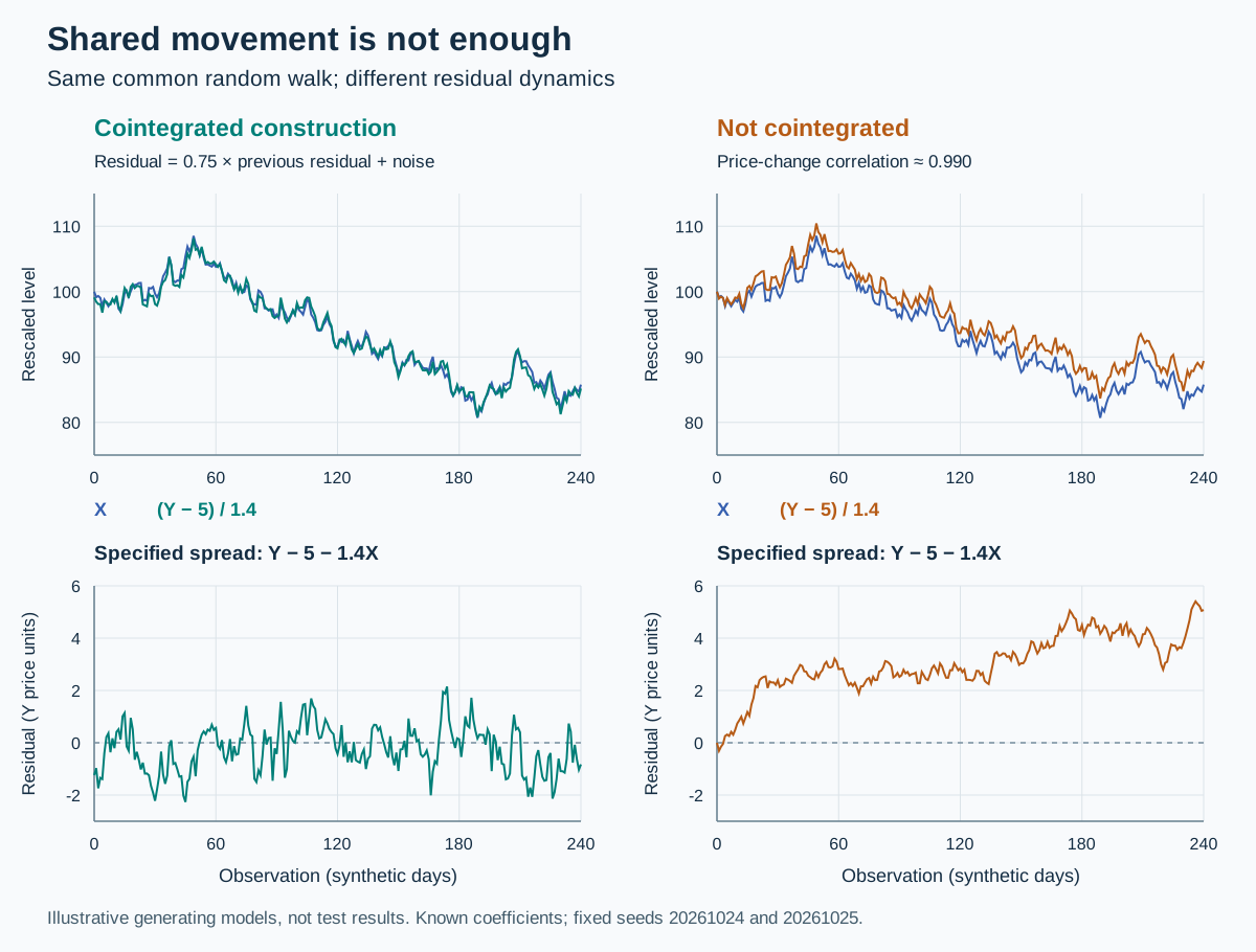
The random walk enters $Y_t$ with coefficient 1.4. Subtracting $5+1.4X_t$ cancels it exactly, leaving the stationary autoregressive residual $z_t$ . Both price levels are $I(1)$ under this model, while their specified combination is $I(0)$ .

For example, if $X=110$ and $Y=161$ , the residual is

z=161-5-1.4(110)=2.

The fitted relationship puts $Y$ at 159, so its observed price is 2 above that reference. Under this particular AR(1) model, the next residual has conditional expectation $0.75\times2=1.50$ . That is an expected adjustment, not a promise about the next observation.

High correlation can leave a wandering spread

Now keep the same $X_t$ , but replace the stationary residual with an independent random walk:

v_t=v_{t-1}+\xi_t,\qquad \widetilde Y_t=5+1.4X_t+v_t,

where $\xi_t$ has standard deviation 0.2 and is independent of $\eta_t$ . Then

\Delta\widetilde Y_t=1.4\eta_t+\xi_t.

The price changes are extremely correlated:

\operatorname{Corr}(\Delta X_t,\Delta\widetilde Y_t) =\frac{1.4}{\sqrt{1.4^2+0.2^2}} \approx0.990.

Yet $\widetilde Y_t-5-1.4X_t=v_t$ is a random walk. Its variance grows with time. More generally, subtracting $bX_t$ leaves $(1.4-b)X_t+v_t$ plus a constant. No fixed $b$ can eliminate both independent stochastic trends, so these two series are not cointegrated.

Two synthetic constructions share the same random-walk driver. In the left panels, rescaled levels move together and their specified spread is stationary. In the right panels, price changes have approximately 0.990 population correlation, but an independent random-walk component makes the spread wander.

Original seeded simulations with 241 observations. Upper panels plot $X$ and the rescaled series $(Y-5)/1.4$ so their shared movement can be compared on one scale. Lower panels show the unscaled residual $Y-5-1.4X$ . The plotted coefficients are the known generating parameters. These charts illustrate the models; they are not empirical cointegration tests.

The distinction also runs in the other direction: cointegration can coexist with weak short-run correlation if stationary, company-specific fluctuations dominate daily changes. Correlation of nonstationary levels can be misleading as well; a visually close fit or a high regression

R^2

can arise in a spurious regression.

Stationary does not mean confined forever inside fixed bands. A Gaussian stationary residual has unbounded support. Large deviations can occur even when its distribution remains stable.

What a test can establish

With actual data, Nadia does not know the correct intercept, coefficient, or residual process in advance. The Engle–Granger two-step method estimates a relationship and tests whether its residual still has a unit root.

Check whether each candidate level series plausibly has the same integration order, usually $I(1)$ . Inspect the data and deterministic terms; failing to reject a unit root is not proof of one.
Fit $Y_t=a+\beta X_t+u_t$ on a formation sample, often using ordinary least squares.
Test the fitted residual with cointegration-specific critical values. The null is no cointegration. An ordinary ADF test p-value on the estimated residual is not the correct Engle–Granger p-value.

The statsmodels cointegration documentation states the

I(1)

assumption, null hypothesis, deterministic specifications, and MacKinnon-based reference values. Its test is a statistical procedure, not a measure of trade profitability. For a basket with several potential relationships, the Johansen procedure addresses the number of independent cointegrating vectors. The Reserve Bank of Australia's test-procedures appendix provides an applied research explanation of both approaches.

Choosing the pair with the smallest p-value from hundreds of candidates creates a multiple-testing problem. Preserve a separate period for out-of-sample evaluation, and specify when coefficients can be re-estimated. A structural break, such as a company changing its business mix, can invalidate a relationship that held historically.

The coefficient's units decide the hedge

In the price-level relationship

z=Y-a-\beta X

, assume both prices are quoted in the same currency per share. Then

\beta

converts an

X

price change into a

Y

price change. For a fixed coefficient, long one share of

Y

and short

\beta

shares of

X

has gross price-change profit

\Delta Y-\beta\Delta X=\Delta z.

For Nadia's coefficient, that is one $Y$ share against 1.4 $X$ shares. The intercept cancels from the change. The identity excludes dividends, financing, borrowing charges, and trading costs; cash and funding still need an explicit ledger.

A log-price relationship is different:

z=\log Y-a-\beta\log X.

Now $\beta$ is an elasticity. For small changes,

dz\approx\frac{dY}{Y}-\beta\frac{dX}{X}.

A local share hedge ratio against one

Y

share is therefore approximately

\beta Y/X

shares of

X

, rather than simply

\beta

. At prices

Y=161

X=110

, and a separately estimated log-model coefficient of 1.4, that ratio would be about 2.049. A price-level coefficient does not automatically carry over to the log model.

These distinctions prevent a statistical spread chart from being mistaken for actual portfolio performance. Even a genuinely stationary residual may adjust too slowly to cover transaction costs and stock-borrow fees. It can move further against a position before reversing. Cointegration identifies a relationship worth investigating; a trade still needs feasible positions, costs, risk limits, and honest evaluation.

Follow the relationship into a worked research process

SelfMadeQuant's The maths of statistical arbitrage: from a fitted spread to a trade is a free public article. It takes a price relationship through regression arithmetic, residual testing, adjustment speed, hedge sizing, and a trade ledger. It is the closest next reading if your question is how the statistical idea becomes an implementable position.

For formal treatment, Cointegration and Error Correction connects residual tests, adjustment equations, and Johansen rank. The public page is a preview; the full lesson requires membership. The Econometrics and Financial Time Series Programme offers the surrounding sequence on stationarity, forecasting, and multivariate models; its syllabus is public and full lessons are for members.