Geometric Brownian motion: Definition & Examples

Geometric Brownian motion (GBM) is a continuous-time model in which a positive variable has constant proportional drift and volatility. For a stock price

S_t

, it is written

dS_t=\mu S_t\,dt+\sigma S_t\,dW_t,\qquad S_0>0,

where

W_t

is Brownian motion. “Geometric” means that shocks scale with the current price: the same percentage shock moves a stock worth 200 twice as many dollars as one worth 100.

GBM gives a useful benchmark for scenario generation and option pricing: its transitions, moments and European option prices are tractable. Its positive prices are a property of the chosen model, rather than evidence that it captures defaults, crashes or changing volatility.

Which growth rate does the model specify?

Start under a physical probability measure

\mathbb{P}

, intended to describe possible real-world outcomes. Here

\mu

is the instantaneous expected price return per unit time. In the example below there are no dividends, so price return is also the shareholder’s total return. With dividend-paying stocks, distinguish price appreciation from total return.

When time is in years, $\mu$ has units $\text{year}^{-1}$ and $\sigma$ has units $\text{year}^{-1/2}$ . Thus $\mu h$ and $\sigma\sqrt h$ are dimensionless for a horizon $h$ measured in years. A quoted 20% annualised volatility means $\sigma=0.20$ on this time scale; it does not make every one-year price move 20%.

Dividing the SDE by

S_t

may tempt you to integrate it as ordinary calculus and write

S_t=S_0e^{\mu t+\sigma W_t}

. That misses the curvature correction. Apply Itô’s lemma to

\log S_t

instead. Since its first two derivatives are

1/S_t

and

-1/S_t^2

\begin{aligned} d\log S_t &=\frac{1}{S_t}\,dS_t-\frac{1}{2S_t^2}\sigma^2S_t^2\,dt\\ &=\left(\mu-\frac{\sigma^2}{2}\right)dt+\sigma\,dW_t. \end{aligned}

Integrating and exponentiating gives the exact solution

S_t=S_0\exp\left[\left(\mu-\frac{\sigma^2}{2}\right)t+\sigma W_t\right].

The proportional price drift is $\mu$ ; the expected log return per year is $\mu-\sigma^2/2$ . Both describe the same process. Hull derives this distinction in §§14.6–14.7.

For constant coefficients, log returns over disjoint intervals are independent. Equal-length intervals also have the same distribution. Dollar price changes are not independent increments: their scale depends on the price reached. Nor are successive price levels independent.

An 8% drift does not promise an 8% gain

Imagine a risk analyst modelling one non-dividend-paying share with these hypothetical physical assumptions:

S_0=100\text{ USD},\qquad \mu=0.08\text{ year}^{-1},\qquad \sigma=0.20\text{ year}^{-1/2},\qquad T=1\text{ year}.

Because $W_1$ is standard normal,

\log(S_1/100)\sim\mathcal{N}(0.06,0.04).

The second parameter of this normal distribution is variance; the log-return standard deviation is

0.20

. The terminal price has a lognormal distribution.

For general $T$ , its moments and median are

\begin{aligned} \mathbb{E}^{\mathbb{P}}[S_T]&=S_0e^{\mu T},\\ \operatorname{median}(S_T)&=S_0e^{(\mu-\sigma^2/2)T},\\ \text{Var}^{\mathbb{P}}(S_T)&=S_0^2e^{2\mu T}(e^{\sigma^2T}-1). \end{aligned}

The resulting one-year quantities answer different questions:

Quantity	Model result	Interpretation
Expected log return	$0.06$	Mean of $\log(S_1/S_0)$
Expected terminal price	USD 108.33	Average across the terminal distribution
Median terminal price	USD 106.18	Half the terminal probability is below this price
Expected simple return	8.3287%	$e^{0.08}-1$ , rather than exactly 8%
Probability of a price loss	38.21%	Probability of finishing below USD 100

To calculate the last row, turn the price event into a normal threshold:

\mathbb{P}(S_1<100) =\mathbb{P}(0.06+0.20Z<0) =\Phi(-0.30) \approx0.382089,

where $Z\sim\mathcal{N}(0,1)$ and $\Phi$ is its cumulative distribution function. Positive expected growth can coexist with a substantial loss probability.

The mean exceeds the median because high-price outcomes pull the average upward. Taking the exponential of the expected log price gives the median here, not the expected value of price. This is the practical effect of the exponential’s convexity, also reflected in Jensen’s inequality. The smooth median curve is not a path that a “typical stock” is required to trace.

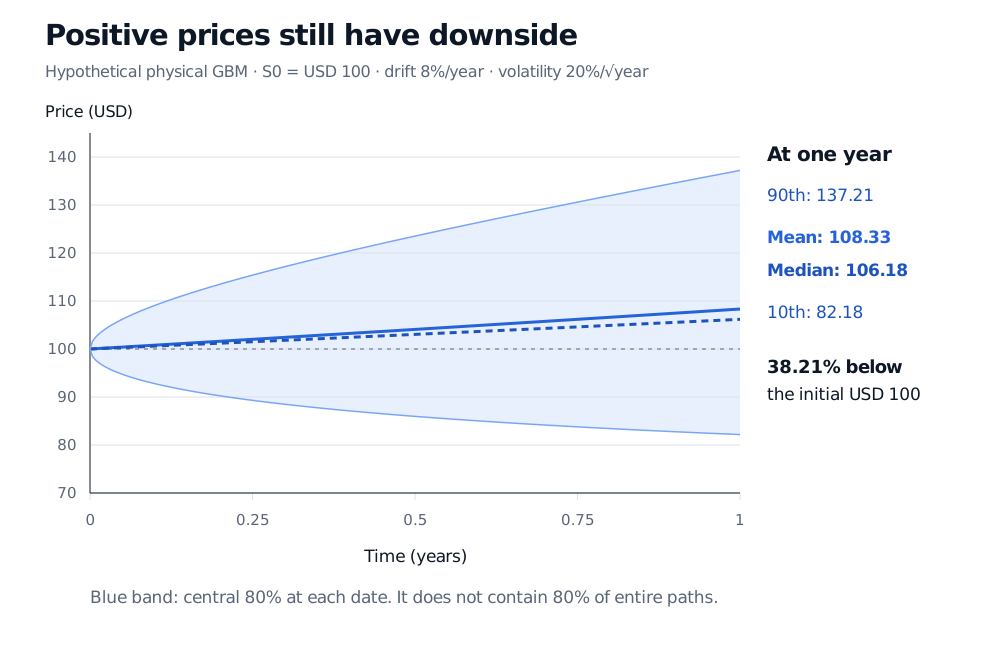
The central 80% GBM marginal band expands from USD 100 to USD 82.18–137.21 at one year; mean 108.33, median 106.18 and probability below the initial price 38.21%.

Analytic model quantiles and moments, not market data or simulated paths. The central 80% band applies separately at each date, not to the probability of staying inside it for the whole year.

Sample the exponential, not its linear approximation

Given the current price and a step of $h>0$ years, draw a fresh independent standard normal $Z$ and use

S_{t+h}=S_t\exp\left[\left(\mu-\frac{\sigma^2}{2}\right)h+\sigma\sqrt h Z\right].

Repeat with independent draws for disjoint intervals. This produces the exact joint GBM distribution at the chosen observation dates. For a payoff depending only on $S_T$ , a single terminal draw suffices. For a discretely monitored Asian payoff, sample the actual averaging dates.

The Euler–Maruyama method instead uses

S_{t+h}^{\mathrm E}=S_t^{\mathrm E}(1+\mu h+\sigma\sqrt h Z).

It is an approximation. For one full-year step in the example, compare the two transformations of the same shock:

Standard normal shock $Z$	Exact price, USD	Euler price, USD
$-2$	71.18	68.00
$0$	106.18	108.00
$2$	158.41	148.00

The zero-shock outcome is the median of each one-step distribution. It need not be its mean. One-step Euler has mean 108; exact GBM has mean 108.33. The errors also change the distribution’s shape, so the direction of an option-price error depends on its payoff and parameters.

For a positive starting value and $\sigma>0$ , Euler can even produce a negative next price when

Z<-\frac{1+\mu h}{\sigma\sqrt h}.

Here the threshold is $-5.4$ for a full-year step: rare, but possible. Exact GBM stays strictly positive at every finite time, almost surely. Clipping Euler’s negative outputs to zero changes the approximation again; it does not recover the lognormal transition.

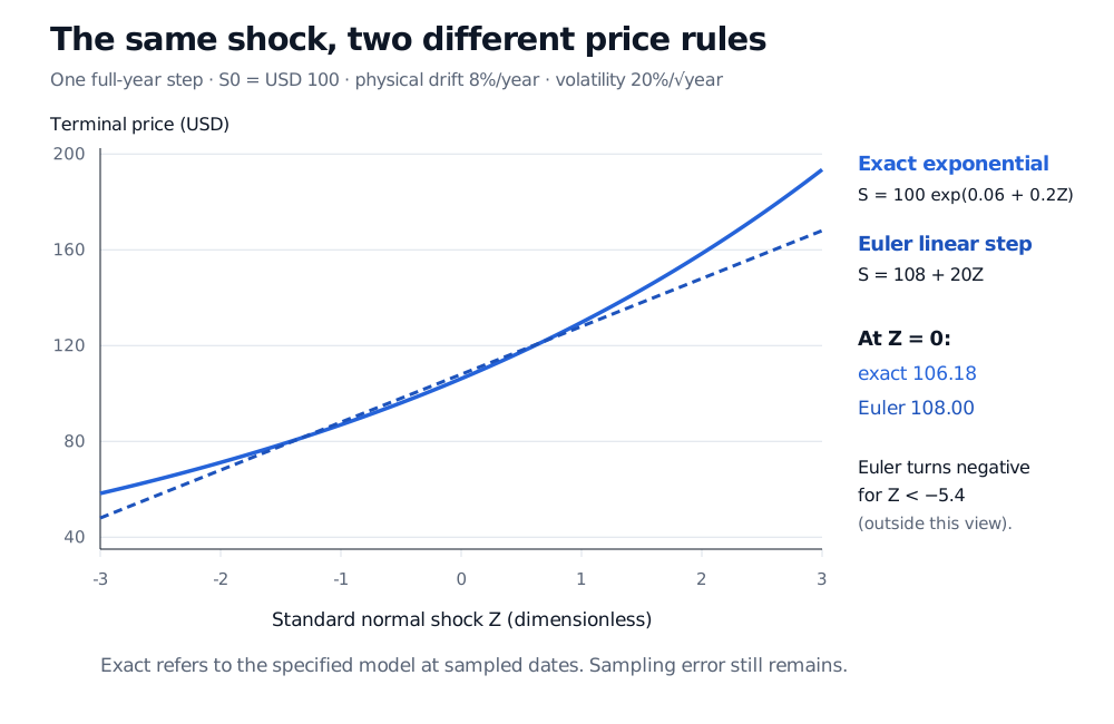
For one year and the same shock Z, exact GBM gives 100 exp(0.06+0.2Z), while Euler gives 108+20Z; their prices and distribution shapes differ.

Original hypothetical one-step comparison. Exponentiation gives the exact GBM transition law; the linear Euler rule changes the distribution. Neither curve is a time path.

“Exact” has a precise scope. A finite Monte Carlo average still has sampling error. Straight lines connecting exact grid values do not reveal intervening barrier crossings. And exact simulation of a chosen GBM does not remove error from choosing that model. The Python GBM walkthrough turns these distinctions into reproducible experiments.

Change the measure before pricing

The risk analyst’s physical drift is an assumption about real-world price growth. In the standard frictionless Black–Scholes framework, risk-neutral valuation uses different probabilities. With constant continuously compounded risk-free rate

r

and continuous dividend yield

q

, the ex-dividend price satisfies

dS_t=(r-q)S_t\,dt+\sigma S_t\,dW_t^{\mathbb{Q}}.

Use $r-q$ in the transition’s price-drift slot, and $r-q-\sigma^2/2$ in its exponent. For example, $r=4\%$ , $q=1\%$ and $\sigma=20\%$ give risk-neutral price drift 3%, log drift 1%, and a one-year mean of USD 103.05 from an initial USD 100. These are valuation-model quantities, not a replacement forecast for the physical example. Haugh’s §§1.1–1.2 derive the pricing measure and dividend adjustment.

For $q=0$ , $e^{-rt}S_t$ is a $\mathbb{Q}$ -martingale. With continuous dividends, use discounted gains including dividends, or the discounted reinvested-total-return value. The discounted ex-dividend stock alone generally is not a martingale.

Where to trust the benchmark

GBM is particularly useful for checking a simulator: does it reproduce the known mean, median and variance under the stated measure? For the derivation, §3.5 of the stochastic-processes lesson and its Exercise 3.3 connect the log transformation with the moment check. The full lesson requires membership; its public page gives a preview.

Challenge the assumptions before using the same benchmark as a risk forecast. Constant volatility excludes volatility clustering; continuous paths exclude jumps. Normal log returns impose specific tail probabilities, which can understate extreme moves in market data. A positive lognormal stock cannot hit zero in finite time, so this model omits a default-to-zero event. Haugh’s §2 discusses jumps, tails and the non-flat volatility surface as limitations of the GBM pricing model.

Increasing the number of simulated paths improves numerical precision conditional on those assumptions. It does not validate the assumed drift, volatility or tails.

Practice: find the drift error

A colleague models a non-dividend-paying stock with $S_0=80$ , $\mu=5\%$ per year, $\sigma=40\%$ per square-root year and $T=0.5$ years under $\mathbb{P}$ . Their simulator uses $80\exp(\mu T+\sigma\sqrt T Z)$ and reports a mean near USD 85.37. Is that consistent with the specified GBM? What should its mean and median be?

Answer. The simulator omitted

-\sigma^2T/2

. Its implemented mean is

80e^{(0.05+0.40^2/2)0.5}=85.37

, so the output can agree with the code while disagreeing with the intended SDE. Correct GBM has mean

80e^{0.05(0.5)}=82.03

and median

80e^{(0.05-0.40^2/2)0.5}=78.81

. The log drift is

-3\%

per year even though proportional price drift is positive. A larger Monte Carlo sample would make the wrong mean more precise.

Sources

John C. Hull, Options, Futures, and Other Derivatives, 9th Global Edition, §§14.3, 14.6–14.7 and 15.1: proportional stock dynamics, Itô’s log transformation and terminal moments.
Karl Sigman, Geometric Brownian motion, Columbia University (2006), §§1.1–1.4: exponential construction, independent price ratios and moments. Sigman uses $\mu$ for log drift; his corresponding proportional price drift is $\mu+\sigma^2/2$ .
Martin Haugh, The Black-Scholes Model, Columbia University (2016), §§1.1–1.2 and §2: risk-neutral dynamics, continuous dividends and GBM’s market limitations.

Which growth rate does the model specify?

An 8% drift does not promise an 8% gain

Sample the exponential, not its linear approximation

Change the measure before pricing

Where to trust the benchmark

Practice: find the drift error

Sources

Related terms

Brownian motion

Expected value

Itô's lemma

Lognormal distribution

Monte Carlo simulation

Normal distribution

Option pricing

Risk-neutral valuation