Itô's lemma: Definition & Examples

Itô's lemma is the chain rule for a smooth function of a continuous stochastic process driven by Brownian motion. It converts a model for a stock price into a model for its logarithm, an option value or another transformed quantity. The distinctive term is a correction for curvature: random fluctuations contribute to the transformed process's drift, even when the fluctuations themselves have zero conditional mean.

That term explains why a stock with an 8% instantaneous expected growth rate need not have an 8% expected log return. It also produces the variance-times-gamma term in the Black–Scholes equation. Before applying the formula, be comfortable with Brownian motion and the distinction between drift and diffusion in stochastic calculus.

A formula you can substitute into

Suppose a continuous Itô process has dynamics

dX_t=a_t\,dt+b_t\,dW_t.

Here $W_t$ is Brownian motion under the chosen probability measure. The coefficients are adapted to the available information, with $\int_0^T(|a_t|+b_t^2)\,dt<\infty$ almost surely on each finite horizon. For a function $f(t,x)$ with a continuous first time derivative and continuous first and second state derivatives, Itô's lemma gives

df(t,X_t)=\left(f_t+a_t f_x+\frac12 b_t^2 f_{xx}\right)dt+b_t f_x\,dW_t.

All derivatives are evaluated at $(t,X_t)$ . This is differential shorthand for an identity between time integrals and an Itô stochastic integral; it does not assume Brownian paths have an ordinary time derivative. Extra integrability is needed when taking expectations of the stochastic integral and setting its mean to zero.

Read the formula in three pieces. Explicit passage of time contributes

f_t

. Movement of the input contributes the ordinary slope term

a_t f_x

. Curvature interacting with instantaneous variance contributes $\tfrac12 b_t^2f_{xx}$ , the Itô correction. The transformed process uses the same Brownian driver, with diffusion coefficient

b_tf_x

; taking a function does not create an independent source of noise. Hull's §14.6 develops this substitution rule.

Why second order survives

A small Brownian increment over $\Delta t$ has scale $\sqrt{\Delta t}$ . Its square therefore has scale $\Delta t$ , so the second-order Taylor term cannot be discarded alongside higher-order terms. For a diffusion, the accumulated squared increments produce quadratic variation

[X]_T=\int_0^T b_t^2\,dt.

This is the meaning behind the calculation rule

(dX_t)^2=b_t^2dt

, and behind

(dW_t)^2=dt

. It is not a pointwise equality for each sampled increment. If

\Delta W=\sqrt{\Delta t}\,Z

, with

Z\sim\mathcal N(0,1)

, then

(\Delta W)^2=\Delta t\,Z^2

, a random quantity. The rule records what remains after squared increments are summed and a suitable grid is refined. MIT's Itô-process notes explicitly introduce the squared-differential notation as a convention.

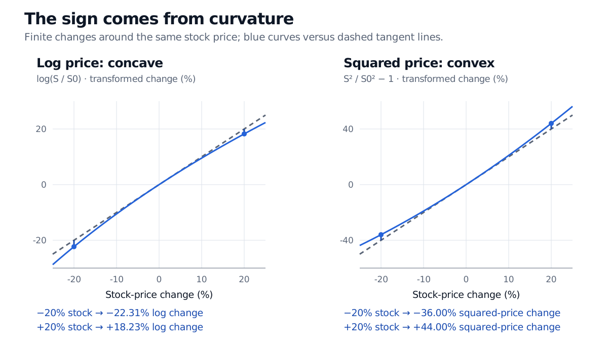
Curvature determines the sign. A convex function lies above its tangent; a concave function lies below it. Symmetric fluctuations therefore have an asymmetric effect after a nonlinear transformation.

Finite stock-price changes illustrate curvature. Logarithms lie below their tangent: minus 20 percent gives a minus 22.31 percent log change, and plus 20 percent gives plus 18.23 percent. Normalised squared prices lie above their tangent: minus 20 percent gives minus 36 percent, and plus 20 percent gives plus 44 percent.

Original function-geometry illustration. The log panel plots $\log(S/S_0)$ ; the square panel plots $S^2/S_0^2-1$ . Blue curves show exact finite changes and dashed lines show first-order tangents. These finite moves illustrate the sign of curvature; they are not a one-year GBM distribution or exact diffusion increments.

One stock model, two different corrections

Use a hypothetical geometric Brownian motion under the physical measure, with time measured in years:

dS_t=0.08S_t\,dt+0.20S_t\,dW_t,\qquad S_0=100.

The price is in USD per share, its drift parameter is $\mu=0.08$ per year, and its volatility is $\sigma=0.20$ per square-root year. These are stipulated model parameters, not estimates from market data.

Log price: subtract half the variance rate

Take $f(S)=\log S$ . Prices remain positive under GBM, so the logarithm is well-defined. Its derivatives are

f_t=0,\qquad f_S=\frac1S,\qquad f_{SS}=-\frac1{S^2}.

Substitute $a_t=0.08S_t$ and $b_t=0.20S_t$ :

\begin{aligned} d\log S_t &=\left[\frac{0.08S_t}{S_t}+\frac12(0.20S_t)^2\left(-\frac1{S_t^2}\right)\right]dt +\frac{0.20S_t}{S_t}\,dW_t\\ &=(0.08-0.02)dt+0.20\,dW_t\\ &=0.06\,dt+0.20\,dW_t. \end{aligned}

The concavity of the logarithm produces a negative correction. Over one year, $\mathbb E[\log(S_1/100)]=0.06$ . This is the expected continuously compounded return, not a statement that the stock's expected one-year simple return is 6%. The different quantities belong to different transformations. Hull's §14.7 derives the same general log-price correction.

Squared price: add a positive variance term

Now take $f(S)=S^2$ . It has $f_S=2S$ and $f_{SS}=2$ , so

\begin{aligned} d(S_t^2) &=\left[2S_t(0.08S_t)+\frac12(0.20S_t)^2(2)\right]dt +2S_t(0.20S_t)\,dW_t\\ &=0.20S_t^2\,dt+0.40S_t^2\,dW_t. \end{aligned}

Here the ordinary chain rule would give a drift coefficient of $2\mu=0.16$ and miss the extra $\sigma^2=0.04$ . At the initial price, the correct instantaneous squared-price drift is $0.20\times100^2=2000$ in squared-price units per year. Squared price is a mathematical risk quantity; this number is not USD 2000 of trading profit.

GBM has the finite moments needed to take expectations here. Writing $m(t)=\mathbb E[S_t^2]$ gives $m'(t)=0.20m(t)$ and hence

\mathbb E[S_1^2]=10000e^{0.20}\approx12214.03.

An independent check uses the exact solution $S_1=100\exp(0.06+0.20Z)$ , with $Z\sim\mathcal N(0,1)$ . Squaring and averaging gives $10000\exp(0.12+\tfrac12\times0.40^2)=10000e^{0.20}$ again.

Do not substitute the square of the expected stock price:

(\mathbb E[S_1])^2=10000e^{0.16}\approx11735.11

. Their difference, approximately

478.92

, is the stock price's variance. Nonlinearity changes the average as well as the dynamics.

Where the correction enters an option hedge

For a smooth option value $V(t,S)$ , write $\Delta=V_S$ and $\Gamma=V_{SS}$ . Under GBM, the formula becomes

dV=\left(V_t+\mu S\Delta+\frac12\sigma^2S^2\Gamma\right)dt +\sigma S\Delta\,dW_t.

A local delta hedge subtracts

\Delta\,dS

from the option's change. The Brownian exposure and the stock's

\mu S\Delta

drift cancel, leaving

dV-\Delta\,dS=\left(V_t+\frac12\sigma^2S^2\Gamma\right)dt.

This is a local gains calculation. A continuously rebalanced, self-financing hedge must also account for its cash financing. For a non-dividend-paying stock in the frictionless Black–Scholes setting, that financing yields

V_t+\frac12\sigma^2S^2V_{SS}+rSV_S-rV=0.

The curvature term survives hedging; the stock's physical expected growth rate does not. Positive gamma alone is therefore insufficient to establish a profitable strategy: time decay, financing, option price and actual trading costs matter. Itô's lemma supplies dynamics; no-arbitrage and replication supply the pricing restriction.

The formula itself also does not change the probability measure. Under risk-neutral GBM with continuous dividend yield $q$ , the stock drift is $r-q$ , while the same curvature correction applies. Multiple risk factors require covariance cross terms; jumps require additional jump terms. A kinked expiry payoff cannot simply be treated as a twice-differentiable function at its strike, although its pre-expiry Black–Scholes price is smooth under the model's usual conditions.

For a longer financial treatment, read §§3.4–3.5 of Stochastic Processes, Brownian Motion and Itô's Lemma: the substitution rule is followed by the exact GBM solution. The public page provides a preview; the full lesson requires membership.

Sources

John C. Hull, Options, Futures, and Other Derivatives, 9th Global Edition, §14.6, equations 14.12–14.14, and §14.7, equations 14.17–14.19 — diffusion transformation and the log-price correction. Numerical examples and figure here are original.
MIT OpenCourseWare, David Gamarnik: Lecture 17, Itô process and formula, 6.265/15.070J, Fall 2013, pp. 1–4 — squared-differential notation, chain rule and Taylor-expansion argument.
Fabrice Baudoin: Lecture 21, Itō's formula, 19 September 2012, Theorems I–III — continuous-semimartingale formulation, explicit time dependence and multidimensional extension.

A formula you can substitute into

Why second order survives

One stock model, two different corrections

Log price: subtract half the variance rate

Squared price: add a positive variance term

Where the correction enters an option hedge

Sources

Related terms

Brownian motion

Delta hedging

Gamma

Geometric Brownian motion

Stochastic calculus

Variance