Brownian motion models continuous random shocks with independent Gaussian increments. Understand time scaling, dependent levels, quadratic variation and what a simulated path can show.
Brownian motion
Brownian motion, also called a Wiener process, is a continuous-time random process with continuous paths and independent Gaussian increments. Standard Brownian motion starts at zero, has zero drift, and accumulates variance at one unit per unit of time. It is a model of the shocks driving many financial models: the noise that is scaled and transformed into prices, rates or portfolio gains.
A Brownian value is not itself a stock price. It can be negative, has no currency units until a model assigns them, and has no built-in expected investment return. Its useful feature is a precise rule for how uncertainty accumulates.
What the definition commits you to
Write standard Brownian motion as (Wt)t≥0. With time measured in years, its defining properties are:
W0=0 almost surely.
For 0≤s<t, the increment has a normal distribution: Wt−Ws∼N(0,t−s). The second argument is variance.
Increments over disjoint time intervals are independent.
With probability one, the entire path is continuous.
Condition 2 includes stationarity of increments: their distribution depends on interval length, rather than the starting calendar date. The levels themselves are not stationary, because Var(Wt)=t grows with time. “Continuous” means there are no jumps; it does not mean smooth.
In financial modelling, we usually specify an information set Fs containing everything available by time s. Calling W Brownian with respect to that information requires Wt−Ws to be independent of Fs. For the process’s own history this follows from the definition; arbitrary extra information might reveal a future shock. The information qualification matters when constructing a stochastic integral.
These are model assumptions, not conclusions from a noisy price chart. A central limit theorem can motivate Gaussian approximations for suitably scaled sums. It does not make an observed sequence of small shocks exactly Gaussian, establish path continuity, or prove that a market is informationally efficient. A process-level limit from random walks needs additional conditions and a functional convergence theorem.
A quarter of a year is half the shock size
For an interval of length h, the exact increment law can be written
An increment above 1 is therefore a two-standard-deviation event. With Φ the standard normal cumulative distribution function,
P(ΔW>1)=1−Φ(0.51)=0.022750131948…
The probability is about 2.275%, regardless of when that quarter-year begins, under the model.
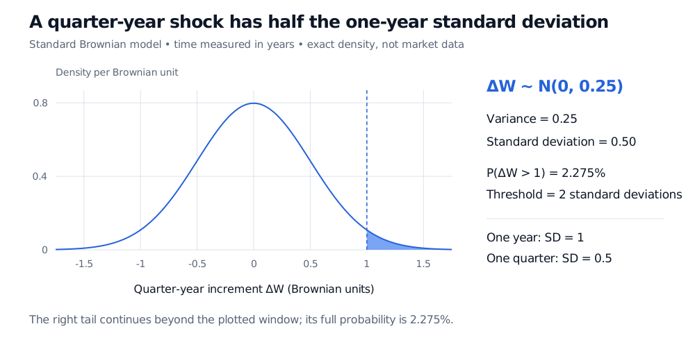
A quarter-year Brownian increment has variance 0.25 and standard deviation 0.5; increments above 1 form the shaded 2.275% right tail.
Original exact model density, with time measured in years. A quarter of the time gives a quarter of the variance and half the standard deviation; the full right-tail probability is 2.275%. The tail continues beyond the plotted window.
To give the shock financial units, suppose an illustrative trading desk models cumulative, zero-drift noise in its profit and loss as
Xt=40Wt,
where Xt is measured in thousands of USD, and the loading 40 has units of thousands of USD per square-root year. The quarter-year noise has standard deviation 400.25=20 thousand USD. A gain above USD 40,000 has the same 2.275% probability calculated above. This deliberately simple arithmetic model permits gains and losses without bounds; it is not a calibrated risk forecast or a positive stock-price model.
The broader Brownian scaling property says that, for a>0, Wat/a is again standard Brownian motion. This is equality in distribution of processes, not a claim that a particular realised path satisfies Wat=aWt. Applying square-root-of-time scaling to market returns additionally assumes the chosen constant-variance Brownian model is appropriate over those horizons.
Independent changes still produce dependent levels
Split a one-year value at the quarter-year mark:
W1=W0.25+(W1−W0.25).
The second term is independent of the first. But W1contains the first term, so the two levels share randomness. In general, for 0<s≤t,
Consequently Cov(Ws,Wt)=min(s,t). Here the covariance of W0.25 and W1 is 0.25, and their correlation is 0.25/(0.5×1)=0.5, not zero.
Given the history up to s, the future level is normal with conditional mean Ws and variance t−s. Equivalently, EWt∣Fs]=Ws: standard Brownian motion is a [martingale for an appropriate filtration. That statement describes the model’s conditional mean. It supplies neither an empirical test of efficiency nor a guarantee that a traded asset’s undiscounted price has zero expected return.
Roughness that survives adding the squares
Brownian paths are continuous but, almost surely, nowhere differentiable. There is no ordinary finite instantaneous slope dWt/dt. The fact that an increment has typical size h explains why dividing it by h becomes problematic as h shrinks; that intuition alone does not prove the simultaneous claim at every time. Lalley’s university notes give the nowhere-differentiability theorem and a proof, §6.2.
A related property makes Itô’s lemma work. On a uniform grid with n intervals over [0,T], let
Qn=i=1∑n(WiT/n−W(i−1)T/n)2.
Independent Gaussian increments give
E[Qn]=T,Var(Qn)=n2T2.
Therefore Qn→T in mean square as n→∞. Almost-sure convergence also holds along the usual nested dyadic grids. This limit is Brownian quadratic variation, written [W]T=T. The symbolic rule (dWt)2=dt summarises this accumulation of squared increments; a single squared random increment is not equal to its interval length.
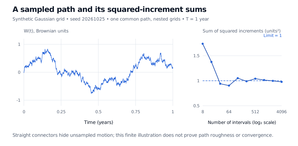
One seeded Gaussian-grid path with 4096 intervals and its nested-grid squared-increment sums; sums fluctuate around the theoretical limit 1.
Original synthetic Gaussian grid, seed 20261025. Nested grids aggregate increments from one common fine path. Dashed line: theoretical limit 1. Straight connectors omit the motion between observations.
Simulation draws independent N(0,T/n) increments and adds them. Those are exact Brownian samples at the grid points. Connecting them with straight lines gives a finite polygon whose slopes exist between vertices. Refining those same straight segments drives its quadratic-variation sums to zero. Revealing further Brownian samples is a different operation. Neither the picture nor one table of sums proves a limiting theorem, and an unobserved barrier crossing can occur between grid points.
In geometric Brownian motion, this noise enters proportionally to the current price. Brownian motion remains the driver; the transformed price is positive and has a different distribution. Jumps, changing volatility and heavy-tailed shocks require richer assumptions. Constant Brownian noise is useful precisely because its restrictions are explicit.
For a continuation, read Definition 3.2, the increment and covariance formulas in Proposition 3.3, and the diffusion definitions in §3.3 of Stochastic Processes, Brownian Motion and Itô’s Lemma. The full lesson requires membership; a public preview shows its outline.
Check the two common confusions
1. Over an interval of 0.09 years, what is P(ΔW>0.3)? If a log-return model has Brownian loading 0.30 per square-root year, what is the standard deviation of its noise over that interval?
Answer. The Brownian increment has variance 0.09 and standard deviation 0.09=0.3. The threshold is one standard deviation, so the probability is 1−Φ(1)=0.158655…, about 15.87%. The log-return noise has standard deviation 0.30×0.3=0.09, or 9 log-percentage points. Multiplying 0.30 by the interval length would incorrectly scale standard deviation linearly.
2. Are W0.4 and W1.6 independent? Find their covariance, correlation and the conditional variance of W1.6 given the history through time 0.4.
Answer. They share the initial 0.4 years of shocks, so they are dependent. Covariance is 0.4 and correlation is 0.4/0.4×1.6=0.5. The independent future increment has variance 1.6−0.4=1.2, which is the conditional variance. Knowing the earlier level removes the uncertainty already realised; it does not remove the next 1.2 years of shocks.
Sources
Gregory F. Lawler, Stochastic Calculus: An Introduction with Applications, revised February 15, 2023, §§2.4, 2.6 and 2.8 — Brownian definition, information sets, covariance, scaling and quadratic variation.
John C. Hull, Options, Futures, and Other Derivatives, 9th Global Edition, §14.2, equations 14.1–14.3 — Wiener increments, variance rates and financial noise loadings.