The central limit theorem (CLT) describes the limiting distribution of a centered, scaled sum of random variables. In its classical form, independent and identically distributed observations with finite, positive variance produce a standardized sum whose distribution approaches the standard normal distribution.
For a quant, this connects the variability of individual simulated payoffs or trade profits to the uncertainty of their average. It does not turn individual returns into normal observations, establish a profitable strategy, or certify a normal model for rare losses.
What is becoming normal?
Let be independent observations from the same distribution, with expected value and variance . Define the sum and sample mean . The theorem states
Here convergence in distribution means that, for every fixed real ,
where is the standard normal cumulative distribution function. The limit concerns probabilities across repeated samples. It does not say the sequence of realized values settles at zero.
The centering and scaling are essential. Under these assumptions, the following moment identities are exact for every sample size, before using any normal approximation:
Thus the sum spreads out while the average concentrates. Standardization puts both on the same unitless scale. The law of large numbers says that the average approaches its mean; the CLT describes the shape of its fluctuations when magnified by . The normal approximation for an unstandardized mean is , with an -dependent variance. MIT's CLT slides illustrate these three equivalent scales.
A hundred trades still have only two single-trade outcomes
Consider a stipulated model, rather than market observations: each trade independently makes USD 6 with probability 0.55, or loses USD 4 with probability 0.45. These dollar profits are assumed to include all costs, with no changing position size, dependence or capital constraint.
The population mean and variance are
One trade's standard deviation is about USD 4.9749. The standard error of the average is much smaller:
| Number of independent trades | Mean profit's standard error, USD per trade |
|---|---|
| 25 | 0.9950 |
| 100 | 0.4975 |
| 400 | 0.2487 |
Quadrupling the count halves this uncertainty scale. It does not guarantee that a particular realized average moves closer to USD 1.50 each time more trades are added.
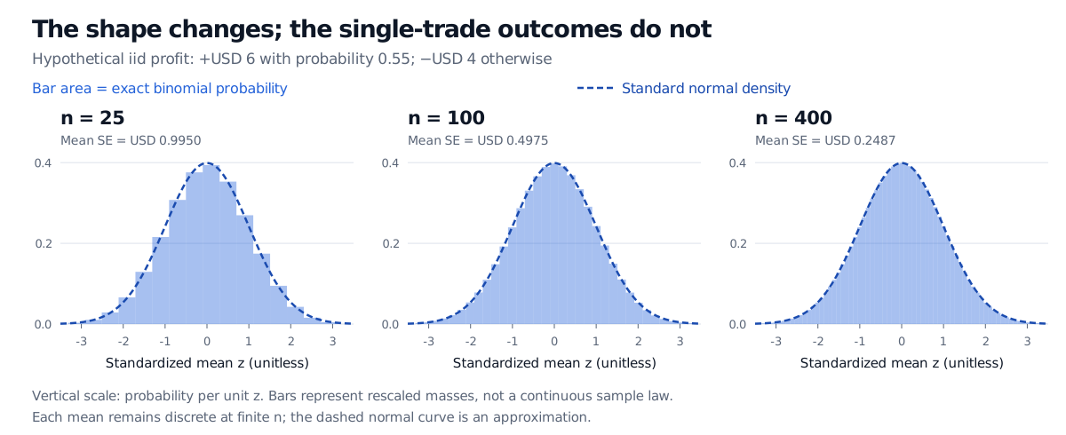
Original hypothetical iid model; exact enumeration. Bar areas are exact probabilities on a common standardized scale. Each finite-sample law remains discrete.
Every individual trade still has the same two possible outcomes. What changes is the distribution of the average across a batch. The bars become finer and their overall shape approaches the dashed normal curve.
Check an approximation against the exact answer
What is the chance that the average profit over 100 trades lies between USD 1 and USD 2, inclusive?
Let count winning trades. Then has a binomial distribution with parameters and , and
The event is therefore . Direct enumeration gives
The corresponding normal count approximation has mean and variance . Because counts are discrete, include the whole unit-width bins around the two boundary outcomes: use 49.5 and 60.5, rather than just 50 and 60. This is the continuity correction:
| Calculation | Probability |
|---|---|
| Exact binomial | 73.1170% |
| Normal with continuity correction | 73.1075% |
| Normal using uncorrected bounds 50 and 60 | 68.5121% |
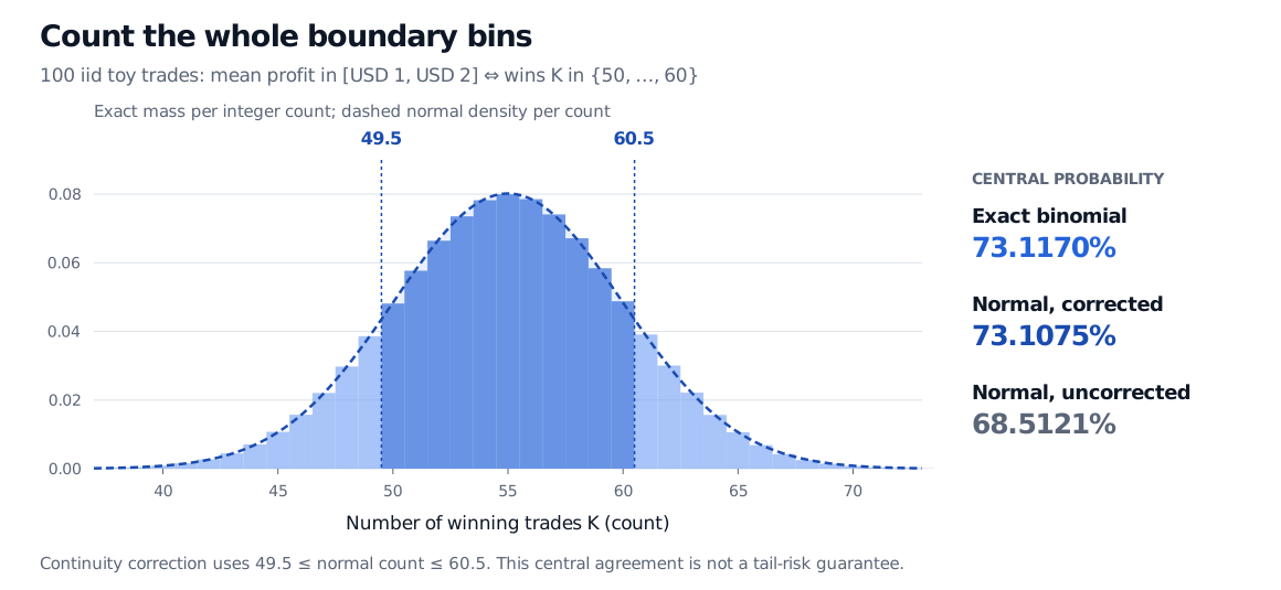
Original hypothetical iid model. Including whole boundary bins makes this central approximation close to the exact answer. It remains an approximation.
The half-unit correction applies to win counts. On the average-profit scale, the lattice spacing is USD 0.10, so the corrected boundaries are USD 0.95 and USD 2.05. Adding half a dollar would use the wrong units.
An error bar needs a clear question
Using the known population parameters, the approximate central 95% sampling band for the 100-trade average is
This predicts where repeated sample averages tend to land around a known mean. Its actual probability in this discrete example is about 94.4370%, because only integer counts 46 through 64 fall within those boundaries. The label “approximate” matters even in this well-behaved model.
When the mean is unknown, a confidence interval instead centers on the observed average. A familiar large-sample interval uses , with estimating the population standard deviation. Its justification and finite-sample coverage need their own checks; substituting estimates does not make an interval exact.
In Monte Carlo simulation, the same logic applies to independent simulated outputs with finite variance. It quantifies sampling noise under the chosen model. More simulations cannot repair a missing crash scenario, a mispriced payoff or a biased trading rule.
Before using it on a return series
Dependence changes the calculation. Under covariance stationarity, writing gives the exact identity
Serial covariance can make the independent-observation standard error too small or too large. Suitable dependent-data CLTs exist, but require additional restrictions on dependence and moments. When applicable, their fluctuation scale can involve the long-run variance . Stationarity alone is insufficient; even summable autocovariances are not a general substitute for the other theorem conditions. Powell's Berkeley notes explain why dependence needs separate assumptions. Volatility clustering can also coexist with zero serial covariance in return levels, so it does not automatically inflate this variance.
There is no universal “30 observations” cutoff. For 100 independent default indicators each with probability 0.001, the count is zero with probability . The distribution is dominated by one atom despite having finite variance and more than 30 observations. The classical theorem is valid as the sample size grows; that does not make its normal approximation useful at every finite size.
Finite variance does not promise accurate far tails. A finite mean with infinite variance can still permit a law of large numbers while falling outside this classical CLT. With finite variance, convergence can be slow. A Berry–Esseen bound adds a quantitative absolute-probability error bound when the third absolute centered moment is finite; DasGupta states the extra condition explicitly. Even a small absolute error may be large relative to a tiny tail probability. Good agreement near the center does not validate extreme-loss capital or a value-at-risk estimate.
For a fuller treatment of convergence, bounds and dependent-loss examples, see Laws of Large Numbers and the Central Limit Theorem. Simulation and Resampling develops the Monte Carlo application. Both offer public previews; their full lessons require membership.
Sources
- Dimitri P. Bertsekas and John N. Tsitsiklis, Introduction to Probability, 2nd edition (2008), §5.4, pp. 274–279: classical CLT, normal approximation and binomial continuity correction. All trade-profit calculations and figures here are original.
- MIT OpenCourseWare, 18.05, Class 06b: Central Limit Theorem, Spring 2022: standardization, sample-average uncertainty and continuity correction.
- Anirban DasGupta, Graduate Probability, §1.29.6: finite-sample normal-approximation error and the additional third-moment assumption in Berry–Esseen.
- James L. Powell, Introduction to Time Series Models, pp. 3–4: dependence conditions and the long-run variance of sample averages.