A confidence interval measures parameter uncertainty through a sampling procedure. Calculate a mean-return t interval, interpret repeated coverage, and distinguish confidence from prediction.
Confidence interval
A confidence interval is a range for an unknown population parameter, calculated by a procedure designed to cover that parameter at a stated rate over repeated samples. For a strategy's expected return, it adds an uncertainty range to the historical average. It can reveal that a seemingly attractive estimate is consistent with a small loss as well as a gain.
The confidence level describes the procedure's coverage. It does not turn the finished interval into a probability distribution for the parameter, establish that a strategy is profitable, or describe the range of tomorrow's returns.
A 25-day record: 12 basis points, plus or minus what?
Suppose a researcher reports 25 daily excess returns for one strategy, measured relative to a matched cash benchmark. These are hypothetical summary statistics before trading costs, with the strategy, sample size and analysis fixed in advance:
Quantity
Decimal-return units
Basis points per day
Sample size
25 observations
—
Sample mean xˉ
0.0012
12 bp
Sample standard deviation s
0.0030
30 bp
Estimated standard error s/n
0.0006
6 bp
One basis point is 0.0001 in decimal-return units. The 30 bp standard deviation measures dispersion across individual days. The 6 bp standard error measures uncertainty in the estimated mean under independent sampling. Substituting one for the other changes the question.
For the calculation, stipulate independent, identically distributed normal returns with a constant unknown mean and positive unknown variance. This is a teaching model, rather than a claim about actual market returns. With
Xˉ=n1i=1∑nXi,S2=n−11i=1∑n(Xi−Xˉ)2,
the statistic
S/nXˉ−μ∼tn−1
has a Student t distribution. The denominator is estimated from the same data, which is why the exact cutoff comes from t, rather than a standard normal distribution. A two-sided 95% interval is
xˉ±tn−1,0.975ns.
Here the degrees of freedom are 25−1=24 and the 97.5th percentile is approximately 2.06389856. The margin of error, meaning the half-width, is
2.06389856×0.0006≈0.0012383391.
Thus the interval is
[−0.0000383391,0.0024383391],
or approximately −0.38 to +24.38 bp per day. The daily mean is estimated at 12 bp, with a margin of error of about 12.38 bp. Zero is inside the range. A positive historical average alone has not established a positive population mean.
This is also the decision from the matching two-sided 5% hypothesis test: its statistic against zero is 12/6=2, below 2.0639, so it does not reject a zero mean. The corresponding p-value is approximately 0.05694. This duality holds because the interval and test use the same model, tails and cutoff; mixing a one-sided test with this two-sided interval would change the comparison.
The range is useful beyond that binary decision. It exposes the precision of the effect estimate. A candidate implementation must also survive costs and model uncertainty, neither of which disappears because a mean interval excludes zero.
The interval moves; the mean does not
Before observing data, both endpoints are random functions of the sample. For a parameter θ, a level-(1−α) confidence procedure satisfies
Pθ(L(X)≤θ≤U(X))≥1−α
throughout its stated model. Exact 95% coverage gives equality at 0.95; some procedures are conservative and cover more often. An approximate interval needs a separate justification for how closely its coverage approaches the target.
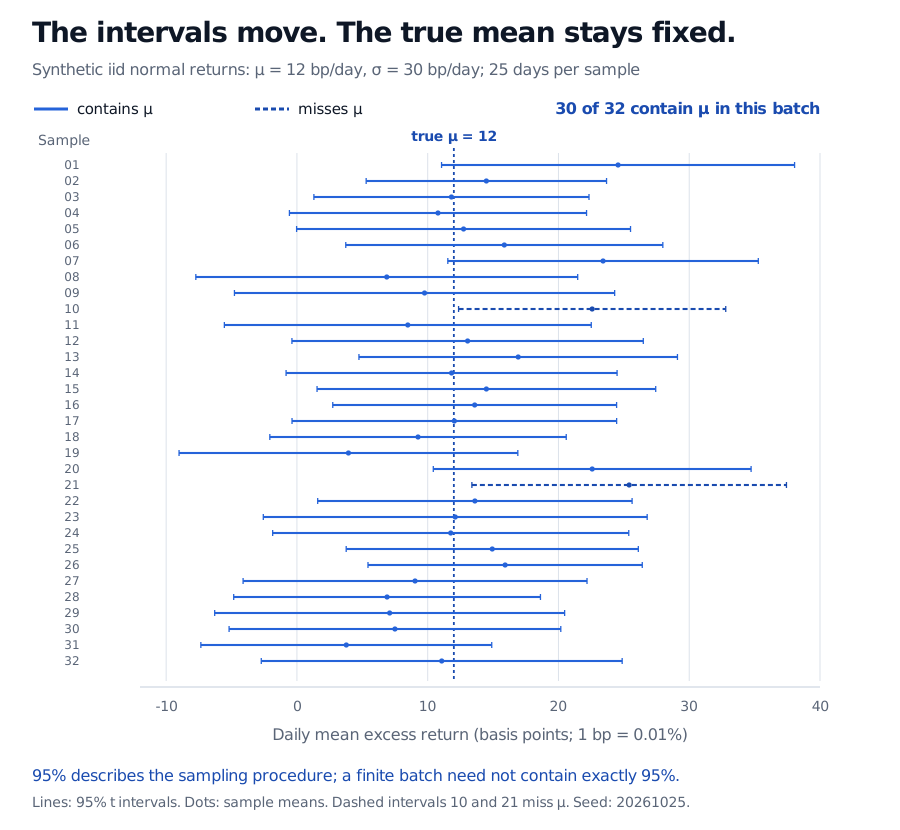
Imagine repeating the entire 25-day experiment using independent samples from the same unchanged return model. Every sample has a different sample mean and sample standard deviation, so the interval shifts and changes length. The underlying mean stays fixed. NIST's coverage explanation associates 95% with this repeated calculation, rather than a probability assigned to the observed endpoints.
Thirty-two independent synthetic normal samples, each with 25 daily returns, produce 95% t intervals. Thirty intervals contain the fixed true mean of 12 basis points per day; samples 10 and 21 miss it. Dots are sample means; dashed intervals indicate misses.
Original seeded iid normal samples: true daily mean 12 bp, standard deviation 30 bp, 25 observations per sample. Thirty of these 32 intervals cover the mean. A finite batch need not deliver exactly 95% coverage.
In this artificial experiment we know the mean because we supplied it to the generator. In real research we do not get to mark the observed interval as a hit or miss. Once calculated, it either contains the fixed parameter or it does not. A statement such as “there is a 95% posterior probability that the mean lies between these endpoints” requires a Bayesian model and a credible interval. It does not follow from frequentist coverage alone, even when particular Bayesian and frequentist endpoints happen to coincide.
A range for the mean is a poor range for tomorrow
The worked interval concerns a population average. A prediction interval concerns a new random outcome. Under the same iid normal model, for one new independent daily return, the 95% prediction interval is
xˉ±tn−1,0.975s1+n1.
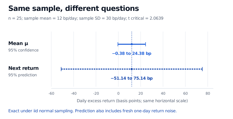
The extra 1 accounts for the new day's return noise; 1/n accounts for estimating the mean. This formula is the single-future-observation case of NIST's prediction limits. For our sample it gives approximately −51.14 to +75.14 bp. Its repeated-sampling guarantee involves both a fresh training sample and a fresh outcome. It does not promise that exactly 95% of all future returns will fall inside this particular realised interval.
On the same daily-return scale, the 95% confidence interval for the mean is −0.38 to 24.38 basis points, while the 95% prediction interval for one new independent return is −51.14 to 75.14 basis points.
Original hypothetical 25-day example under iid normal sampling with unknown mean and variance. Prediction includes fresh one-day noise as well as mean-estimation uncertainty.
With known model parameters, a central probability interval such as [μ−1.96σ,μ+1.96σ] for a normal observation is another distinct object: it describes an outcome distribution, without estimating an unknown parameter. Likewise, a smaller mean margin of error does not imply lower future volatility. More independent data can sharpen the estimate of an unchanged, volatile process.
When the printed 95% stops being the relevant guarantee
The exact t argument needs the sampling model stated above. At 25 observations, replacing normality with a vague claim that the sample is “large enough” is insufficient. A central limit theorem may justify an asymptotic interval under suitable conditions; heavy tails, extreme observations and dependence affect whether that approximation is useful. Bootstrap intervals have their own sampling assumptions too.
For covariance-stationary returns with finite variance, write γk for lag-kcovariance. The actual variance of an average is
Var(Xˉ)=n1[γ0+2k=1∑n−1(1−nk)γk].
The iid formula removes every nonzero-lag term. Positive serial covariance can therefore make s/n too small. Volatility clustering alone does not prove positive return autocovariance, but it does break the exact iid normal justification. A suitable time-series variance estimator or dependence-preserving resampling method needs its own conditions. Regime change can also undermine the premise that one stable mean is being estimated.
Finally, the analysis rule is part of the procedure. Twenty independent intervals, each with exact 95% coverage, have probability 1−0.9520≈64.15% of at least one miss. Correlated strategies need a different joint calculation; individual 95% intervals still supply no automatic simultaneous guarantee. Selecting the most attractive result after a broad search adds overfitting and selection concerns.
Repeatedly extending a backtest until the lower endpoint first becomes positive changes the stopping rule too. Ordinary fixed-sample intervals do not automatically retain 95% coverage at that chosen stopping time. A sequentially valid construction, such as the confidence sequences studied by Howard and coauthors, supplies a different, time-uniform guarantee under explicit assumptions.
Dimitri P. Bertsekas and John N. Tsitsiklis, Introduction to Probability, 2nd ed. (Athena Scientific, 2008), §9.1, pp. 468–472: confidence procedures, repeated-sampling interpretation, estimated variance and the Student t construction. The financial examples and seeded samples here are original.