Expected return: Definition & Examples

Expected return is the probability-weighted average of an investment’s possible returns over a specified horizon. It answers “what is the mean return under these assumptions?” A positive answer does not promise a profit, identify the most likely outcome or describe how quickly one account will compound.

A portfolio manager needs that distinction before deciding how much capital to allocate. An investment can have a positive mean and still lose money in a substantial fraction of scenarios. The mean is one input to the decision; the distribution around it determines how uncomfortable, or unaffordable, the investment could become.

Three possible years

Suppose an investor puts USD 10,000 into a hypothetical investment for one year. There are no additional deposits or withdrawals. The scenario returns include all investment income and price changes, but exclude fees and taxes. The probabilities are stipulated for teaching; they are not estimated market forecasts.

One-year outcome	Probability	Simple return	Terminal wealth	Contribution to expected return
Strong year	20%	+20%	USD 12,000	+4 percentage points
Modest year	50%	+5%	USD 10,500	+2.5 percentage points
Losing year	30%	−10%	USD 9,000	−3 percentage points

The probabilities sum to one. Apply the definition of expected value to the return

R

\mu=\mathbb{E}[R]=\sum_{i=1}^{m}p_i r_i =0.20(0.20)+0.50(0.05)+0.30(-0.10) =0.035=3.5\%.

The first 0.20 is a probability; the second is a return expressed as a decimal. Their product is 0.04, or four percentage points of contribution to the mean. Averaging the three returns with equal weights would give 5%, but that would silently replace the stated probabilities with equal probabilities.

Hypothetical one-year returns +20%, +5% and −10% have probabilities 20%, 50% and 30%. Their contributions +4, +2.5 and −3 percentage points sum to a mean of 3.5%, alongside a 30% chance of loss.

Original hypothetical one-year USD return distribution, before fees and taxes. Bars show probability times return in percentage points, rather than realised returns.

Here the 3.5% mean is not even a possible realised return: the model allows only +20%, +5% or −10%. The most likely outcome is +5%, and the probability of a negative return is 30%. Neither number can be recovered from the mean alone. Variance and standard deviation describe spread, while loss probabilities and tail scenarios answer different risk questions.

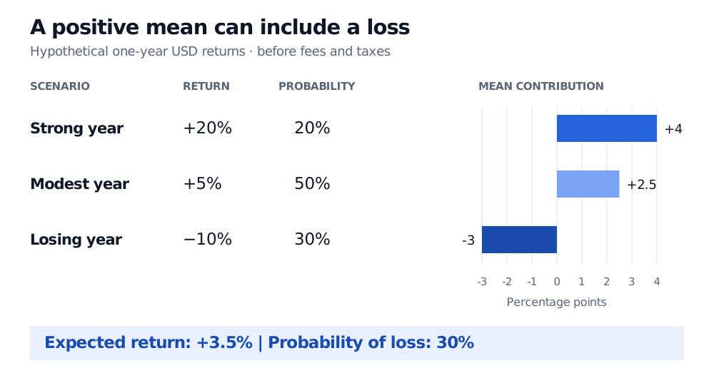
Why expected wealth is USD 10,350

For a fixed initial amount $W_0$ , and terminal wealth $W_1=W_0(1+R)$ , linearity gives

\mathbb{E}[W_1]=W_0(1+\mathbb{E}[R]) =10{,}000(1.035)=10{,}350.

An alternative calculation weights the terminal balances directly:

0.20(12{,}000)+0.50(10{,}500)+0.30(9{,}000)=10{,}350.

This is an expected gain of USD 350, not an amount the investor is owed. Imagining ten otherwise identical investors, with two strong years, five modest years and three losing years, produces the same average balance. That small cohort is an arithmetic illustration, not a prediction that ten independent investments must realise those exact counts.

A forecast mean and a historical average have different jobs

The table specifies a population distribution: outcomes and their probabilities define the mean. In practice that distribution is unknown. An analyst might estimate it from historical returns, economic scenarios or an asset-pricing model.

For $n$ observed returns measured over equal periods, the historical arithmetic mean is

\bar R=\frac{1}{n}\sum_{t=1}^{n}R_t.

That is a sample statistic. Under an independent, identically distributed model with a finite mean, it estimates the common expected return; a finite sample still has estimation error. A long record also cannot ensure that the future distribution will match the past. Changing borrowing costs, strategy crowding or a different business model can change the relevant mean.

A useful forecast therefore states its information set and horizon: expected return conditional on what is known today. A CAPM estimate, for example, adds assumptions about how exposure to market risk is rewarded. It does not convert an expected return into a certain payment. Backtest averages require particular care about look-ahead bias, omitted failed investments and costs.

Compounding asks another question

The arithmetic mean concerns a single period’s simple return. A realised multiyear account grows by multiplying gross returns, $1+R_t$ . With no external flows and equal one-year periods, its compound annual growth rate is

\text{CAGR}=\left(\prod_{t=1}^{n}(1+R_t)\right)^{1/n}-1.

CAGR summarises one realised path. It is not the same object as the forward mean $\mathbb{E}[R]$ .

The scenario model also allows an expected log return, because every gross return is positive:

\begin{aligned} \mathbb{E}[\ln(1+R)] &=0.20\ln(1.20)+0.50\ln(1.05)+0.30\ln(0.90)\\ &\approx0.0292512. \end{aligned}

Exponentiating gives a growth-equivalent simple rate of about 2.97%. Under repeated independent years with this unchanged distribution and full reinvestment, the long-run realised compound growth rate converges to that rate. This is a model result under those assumptions, not a guaranteed future CAGR. The expected log return itself is approximately 0.02925 in log units per year; calling it a 3.5% simple return would mix conventions.

There is no contradiction between 2.97% compound growth and a 3.5% one-year mean. Taking a logarithm before averaging changes the quantity. Likewise, under those independent repeated-year assumptions, expected terminal wealth after several years uses the arithmetic mean, while a typical long-run compounded path is governed by the log mean. Averaging wealth across possible paths and compounding along one path answer different questions.

Specify what the return includes

A return number needs a horizon, currency and accounting basis. “Expected return of 3.5%” is incomplete unless those are clear. A one-month mean cannot automatically be multiplied by twelve to obtain an annual simple-return mean; compounding and dependence across months matter. A USD return can differ from the same investment’s return after conversion into another currency.

Dividend yield covers income relative to price; total return also includes price changes. A yield quote is therefore not interchangeable with an expected total return. Inflation similarly separates nominal returns from purchasing-power returns.

Costs belong inside the calculation. If this example adds a certain USD 100 fee paid at year-end, the fee is 1% of initial capital in every scenario. Expected net return becomes 2.5%, and expected net terminal wealth becomes USD 10,250. That subtraction works because the fee is fixed on the declared basis. A fee charged on terminal assets, performance fees or path-dependent trading costs need their own scenario calculations. The SEC’s fees bulletin explains how transaction and ongoing charges reduce the amount left invested.

For the underlying mathematics, Expectation, Variance and Covariance develops means alongside risk and portfolio co-movement. The public page provides a preview; the full lesson is free with a signed-in account.

Sources

Dimitri P. Bertsekas and John N. Tsitsiklis, Introduction to Probability, 2nd edition (2008), §2.4, “Expectation, Mean, and Variance”: probability-weighted expectation and its interpretation.
John C. Hull, Options, Futures, and Other Derivatives, 9th edition, Global Edition, §15.3, “The Expected Return,” and Business Snapshot 15.1: the distinction between arithmetic returns, expected continuously compounded returns and realised compound performance. The discrete scenarios above are original and do not assume Hull’s continuous-time stock model.
OpenStax, Principles of Finance, §15.1: total return includes income and capital gains; historical arithmetic averages differ from geometric growth.
SEC, “How Fees and Expenses Affect Your Investment Portfolio”, July 23, 2025: transaction and ongoing fees reduce investment returns.

Three possible years

Why expected wealth is USD 10,350

A forecast mean and a historical average have different jobs

Compounding asks another question

Specify what the return includes

Sources

Related terms

Capital asset pricing model

Dividend yield

Expected value

Look-ahead bias

Standard deviation

Variance