Detect future information in backtests: align usable inputs, fitted transformations, completed labels, decision times and feasible trade returns.
Look-ahead bias
Look-ahead bias occurs when a historical decision uses information that would not yet have been available to the strategy making it. A profitable backtest can then reward a trader for knowing a closing price, revised earnings figure or future outcome before it was knowable. The calculation may be arithmetically correct while the trading policy is impossible.
The useful question is more precise than “did I use future rows?”: What could this particular system know, and what could it do, at this particular instant? A row carrying an old calendar date can still contain a later revision. A model coefficient can carry information from future rows even when the trading signal itself has been shifted.
A winning return on a losing trade
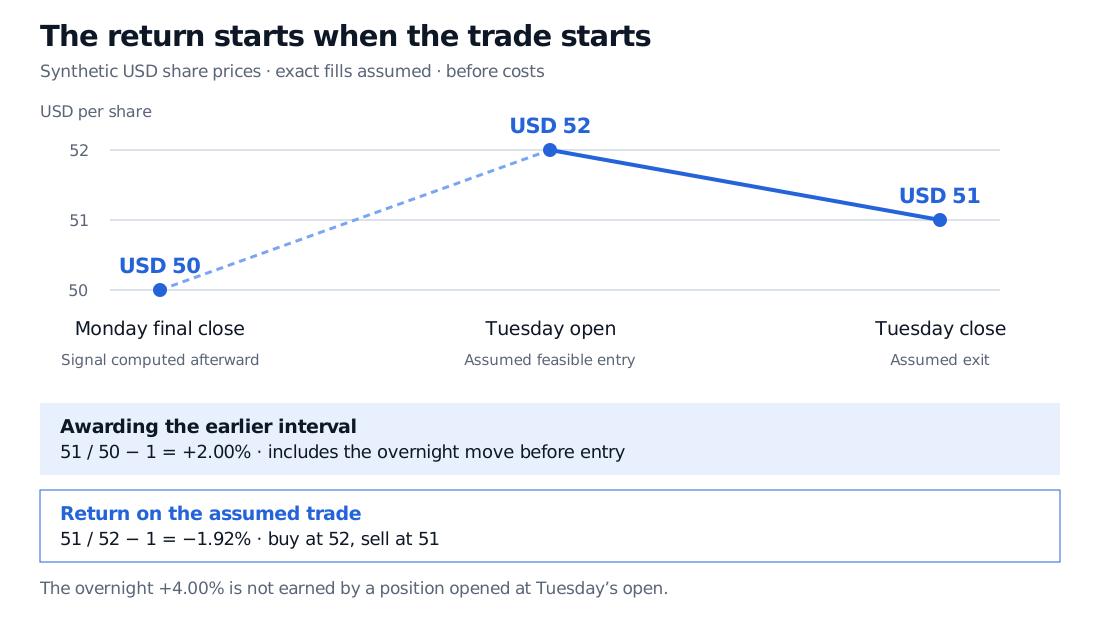
Suppose a hypothetical equity signal needs Monday's final closing price, USD 50. It becomes bullish after that price has been finalised. The strategy is ready before Tuesday's opening auction and, for this simplified example, buys at the Tuesday open of USD 52 and sells at the Tuesday close of USD 51. Assume these fills are feasible, with no dividends, financing or transaction costs.
The return on the assumed holding period is
Rtrade=5251−52=−521≈−1.92%.
A faulty backtest attaches the bullish signal to Monday's close and reports
Rbiased=5051−50=+2.00%.
It has awarded the position Monday's close-to-Tuesday-open move, even though the position did not yet exist. The overnight move was +4.00%; compounding it with the subsequent loss gives the +2.00% close-to-close return. Simply subtracting the two segment returns is not the compounding rule.
Synthetic prices are USD 50 at Monday's final close, USD 52 at Tuesday's open and USD 51 at Tuesday's close. The assumed Tuesday trade loses 1.92%; the biased earlier interval reports a 2.00% gain.
Original hypothetical example, USD per share and simple holding-period returns before costs. Dashed and solid lines connect discrete observations; they do not represent observed intraday paths.
A strategy that genuinely submits a closing-auction order is a different policy. Its signal must use inputs available before its order deadline. It cannot first observe the final auction price and then obtain an earlier guaranteed fill at that price. Moving the signal backward on a spreadsheet does not create that opportunity.
A date is not an information set
Several clocks can legitimately describe one record:
Clock
What it means
Why the distinction matters
Reference or observation time
The period or event measured
Quarter-end is not the earnings release date.
Publication time
When the issuer, exchange or agency releases it
The strategy may receive the publication later.
Receipt time
When the specified system receives it
A message may still require validation or parsing.
Usable time
When the required processing is complete
This is the input's eligibility time for that system.
These labels are a declared data contract; vendors do not universally use the same names. Inspect field definitions, timezones, precision and version identifiers. Two events displayed as “09:30:00” need not be simultaneous. A date-only release field cannot justify a millisecond execution claim.
For an original synthetic revision example, suppose a statistic describing an earlier month first becomes usable on day 10 at 4.2 and is revised on day 20 to 3.8. A decision on day 15 can use 4.2, not 3.8; before day 10 neither version is eligible. A present-day download may contain only the revised number. The St. Louis Fed's real-time-period documentation distinguishes information about the past available today from information known during a historical period. Historical vintages help reconstruct that distinction; they do not establish a particular trading system's intraday receipt latency.
Follow the slowest required input
Let input j become usable at time aj. Under a serial contract with computation delay ℓc and routing delay ℓr, the decision-completion time d, order-arrival time o and fill time f must satisfy
d≥jmaxaj+ℓc,o≥d+ℓr,f≥o.
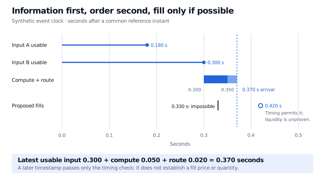
If the latest required input is usable 0.300 seconds after a common reference instant, calculation takes 0.050 seconds and routing takes 0.020 seconds, the earliest order arrival is 0.370 seconds. A simulated fill at 0.330 seconds violates the contract. A fill at 0.420 seconds passes this ordering test, but still needs a defensible price, quantity and execution rule. A later timestamp cannot prove available liquidity or queue priority.
Synthetic event clock: input A is usable at 0.180 seconds, input B at 0.300 seconds; computation finishes at 0.350 and earliest order arrival is 0.370. A 0.330-second fill is impossible; 0.420 seconds is only temporally eligible.
Original serial timing construction, in seconds after one reference instant. The fill markers test causal ordering, not execution availability.
Revised inputs. Joining accounts or macroeconomic releases by the period they describe assigns later knowledge to earlier decisions. Preserve record versions and choose the latest one actually eligible at the cutoff. A backward as-of join needs the right availability field, stable entity identifiers and an explicit stale-data policy.
Fitted transformations. A full-sample mean, imputation rule, regression coefficient, principal-component basis or selected feature can import future information into every historical row. Fit each learned transformation using only the eligible training data, then apply that fitted state to the next decision block. The scikit-learn leakage guidance explains why preprocessing and feature selection belong inside the training boundary. A pipeline helps enforce that boundary; it does not automatically supply a valid chronological split.
Unfinished outcomes. A five-session return label is unavailable when only two sessions have elapsed. At a training cutoff, retain only labels whose full outcome and required processing are complete. Shuffling dated rows can allow later outcomes to influence earlier predictions; a chronological split also needs correct label-availability rules.
Future-selected universes and research choices. Today's surviving stocks can import future survival into a historical universe: survivorship bias is closely related but deserves its own universe audit. Choosing parameters after examining the eventual test performance introduces research-selection bias and overfitting. A correctly lagged signal does not make that test untouched again.
Repair the dependency, then rerun the economics
One-row shifting is useful for a correctly ordered daily series when it matches the intended entry policy. It is not a universal repair for revised data, multi-security panels, irregular events, centred windows or future-fitted model state. Specify the actual dependency and its usable time first.
A practical audit preserves the raw vintage, input versions, transformation state, decision, submitted order and assumed fill for selected historical trades. Check the timing inequalities and align the performance interval with the feasible position. Then rerun with later observations removed: with the same historical snapshot and initial state, earlier frozen decisions should remain identical.
That truncation test can reveal a full-sample transformation or forward window. Passing it does not prove cleanliness: both runs might use the same already revised history. Pair it with vintage inspection and, where available, prospective receipt logs. The Point-in-Time Data lesson works through version selection and the limits of this check (public preview; membership for the full lesson).
Correcting leakage can change both the trades and their measured returns. Rebuild the result from the corrected inputs and feasible fills; adding a small performance haircut cannot undo a decision that used the future. The corrected backtest is a more credible experiment, although it still needs cost, capacity and out-of-sample assessment.
Sources
Ernest P. Chan, Quantitative Trading: How to Build Your Own Algorithmic Trading Business (Wiley, 2009), Chapter 3, “Look-Ahead Bias,” pp. 51–52. Local text checked for whole-sample regression leakage and truncation diagnostics; the examples and clock construction above are original.