CAPM links equilibrium expected excess return to market beta. Work through a 10.2% hurdle rate, separate beta from volatility, and distinguish pricing restrictions from regression fits.
Capital asset pricing model
The capital asset pricing model (CAPM) is an equilibrium model that relates an asset's expected return to its exposure to market risk. Its central restriction is that expected excess return equals market beta multiplied by the expected market excess return. It supplies a benchmark for cost of equity and investment performance; it does not promise the return an investor will receive next year.
The model asks a portfolio question about an individual asset: how much risk does it add when investors already hold a diversified market portfolio? That leads to a different answer from ranking stocks by their standalone volatility.
A hurdle rate before the year begins
An investment committee is evaluating a hypothetical equity investment. Use one-year simple total returns, in the same currency, with a matched risk-free investment earning 3% over that year. Assume the expected market return is 9% and the equity's market beta is 1.2. These are stipulated inputs, not current market estimates.
Write Ri for the asset's random return, RM for the market return and Rf for the known risk-free return. CAPM states
E[Ri]−Rf=βi(E[RM]−Rf).
The expected market premium is 9%−3%=6%, so
E[Ri]=3%+1.2(9%−3%)=10.2%.
The 7.2 percentage point expected excess return compensates for the model's priced market exposure. The extra 3% is the return available on the risk-free investment. For an equity valuation, the committee might use 10.2% as a model-based cost of equity, provided the beta, horizon, currency and cash-flow risk fit the project. It is an estimated required return, rather than an independently observed price of risk.
Now the year ends and the equity has actually earned 12%. The difference from the earlier CAPM benchmark is 1.8 percentage points. That is a one-period comparison with an expected return. It does not establish a persistent alpha, investment skill, or a breach of the model. The realised market return may also have differed from its 9% expectation. A regression residual instead compares the realised asset excess return with a fitted intercept and beta times the realised market excess return.
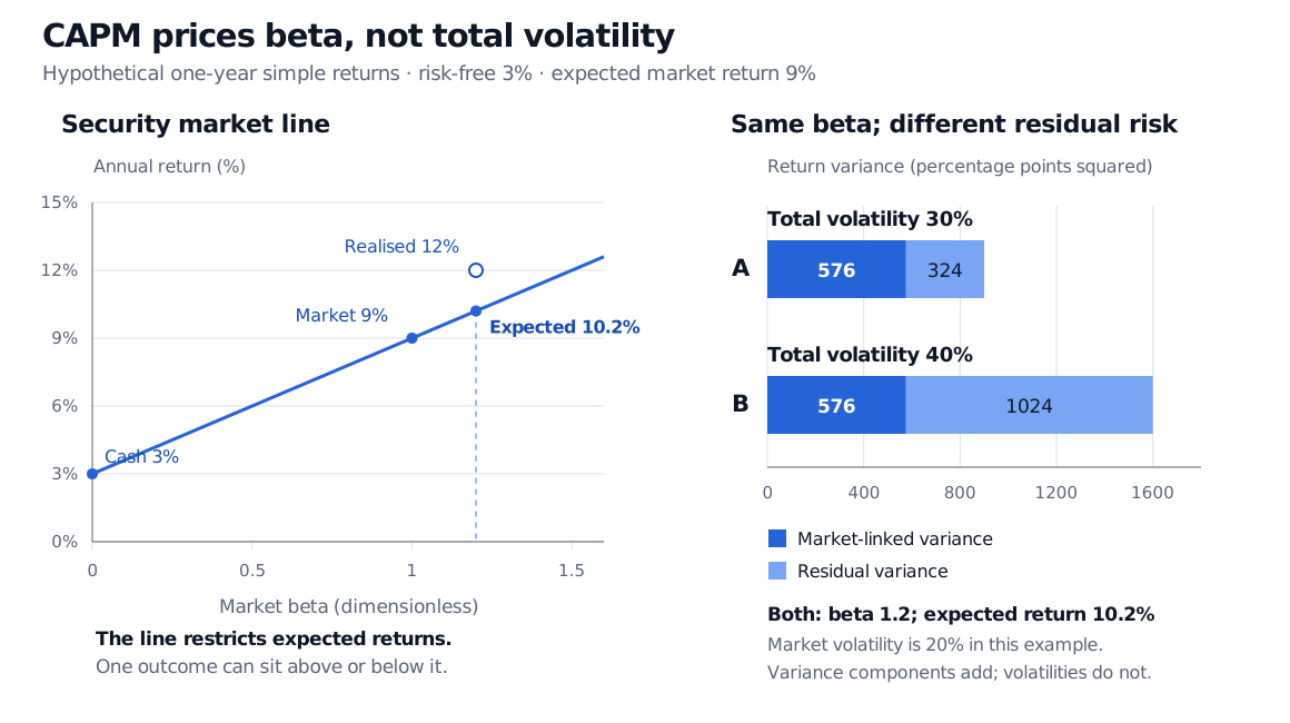
The security market line gives expected return 3% plus beta times 6%, reaching 10.2% at beta 1.2. A separate hollow point shows realised return 12%. Assets A and B both have beta 1.2 and expected return 10.2%, but total volatility is 30% and 40%; their common market-linked variance is 576 percentage points squared.
Original hypothetical annual simple-return example. The line concerns expectations. In the variance panel, market volatility is 20%; market-linked and residual variances add, while their standard deviations do not.
Why covariance enters the price of risk
With positive market variance, beta is
βi=Var(RM)Cov(Ri,RM)=ρiMσMσi.
Here covariance measures joint variation, correlation is its normalised form, and σi,σM are return standard deviations. Beta is dimensionless. It is neither the asset's volatility nor its correlation alone: relative scale matters too. If market variance is zero, the ratio is undefined.
Consider two hypothetical assets consistent with the figure. Both have beta 1.2 against a market with volatility 20%:
Annual population quantity
Asset A
Asset B
Total return volatility
30%
40%
Correlation with market
0.8
0.6
Beta
1.2
1.2
CAPM expected return
10.2%
10.2%
Indeed, 0.8(0.30/0.20)=0.6(0.40/0.20)=1.2. B fluctuates more overall, yet CAPM assigns it no extra expected return. Its extra variation is residual to the market exposure.
To make this precise, form the population linear projection
Ri−E[Ri]=βi(RM−E[RM])+εi,Cov(εi,RM)=0.
Then
σi2=βi2σM2+σεi2.
The common market-linked standard deviation is 1.2(20%)=24%. Residual standard deviations of 18% and 32% give total volatilities of 30% and 40%, since 0.242+0.182=0.302 and 0.242+0.322=0.402. Adding 24% and 18% would be incorrect.
This projection identity holds without CAPM. Uncorrelated residuals need not be independent, and residuals across different assets need not be mutually uncorrelated. Calling all residual variation diversifiable requires more than fitting one regression. CAPM's economic claim is that the market covariance determines the equilibrium premium; it does not erase the losses a concentrated investor can suffer.
Three diagrams with different jobs
The security market line (SML) plots expected return against beta. Under CAPM, every asset and portfolio satisfies this line, including inefficient portfolios. A beta-zero asset has expected return Rf under the model but can still be risky. With a positive market premium, negative-beta assets have expected returns below Rf because their hedge exposure is valuable.
The risky-asset efficient frontier instead plots expected return against total standard deviation. It describes the best available portfolios for specified expected returns, covariances and investment constraints; constructing it does not establish CAPM.
The capital market line (CML) is the efficient boundary formed from the risk-free asset and the tangency portfolio, assuming a common borrowing and lending rate. In standard CAPM equilibrium that tangency portfolio is the market. The CML uses total standard deviation and applies to efficient combinations. An individual stock can lie below the CML while sitting exactly on the SML. Extra residual variance pushes it away from efficiency without creating a higher equilibrium expected return.
The connection is market clearing. In the standard setting, investors agree on return moments and choose the same optimal risky portfolio, changing their risk through cash or borrowing. Aggregate holdings must equal the outstanding market portfolio. The optimality conditions then make expected excess returns proportional to covariance with that portfolio. Elton and coauthors develop these steps in Chapter 13.
An equal-beta trade is not automatically a risk-free arbitrage. Buying one stock and shorting another can cancel estimated market exposure while leaving substantial residual risk. An analyst's forecast above the SML expresses disagreement with a model benchmark; it does not supply a guaranteed profit.
What the equation leaves outside
The standard single-period model assumes mean–variance investors with a common horizon and common expectations, competitive frictionless trading, divisible marketable assets, and access to borrowing and lending at the same risk-free rate. Its unconstrained formulation permits the positions needed for portfolio optimisation. These assumptions support the aggregation argument; taxes, trading costs, borrowing limits, heterogeneous beliefs and nontraded wealth can change it. Sharpe's original paper sets out the move from investor choice to market equilibrium.
Empirical work adds a measurement problem. The theoretical market contains the relevant aggregate risky wealth. A stock index is an observable proxy, not that entire portfolio. Estimated betas depend on the proxy, observation frequency, window and changing exposures. Expected market premia are uncertain too; inserting last year's realised market return changes the question.
A linear regression can estimate a market slope even when CAPM is false. The additional CAPM restriction is a zero population intercept in the correctly specified excess-return projection, across assets, with the appropriate market portfolio. Sample intercepts fluctuate, so testing needs uncertainty estimates and a suitable joint design. A strong fit for one stock does not prove equilibrium pricing. Fama and French's review documents empirical shortcomings and explains why the market-proxy problem affects applications as well as tests.
For the algebraic path from tangency optimality to beta pricing, read Steps 1–3 of Derivation — CAPM from Portfolio Theory. The public page provides a preview; the full lesson requires membership. Read those steps as a derivation conditional on the model's assumptions, then use the distinctions above when interpreting data.
Sources
Edwin J. Elton, Martin J. Gruber, Stephen J. Brown and William N. Goetzmann, Modern Portfolio Theory and Investment Analysis, 9th edition (2014), Chapter 13, especially assumptions pp. 290–291, equilibrium and SML pp. 292–300. The numerical scenario and figures here are original. The explanation uses portfolio optimality rather than the chapter's informal equal-beta arbitrage shortcut.