Efficient frontier: Definition & Examples

The efficient frontier is the set of feasible portfolios for which no other feasible portfolio has at least as high an expected return and at most as much return volatility, with one strict improvement. It is a boundary of choices under specified inputs and trading constraints. It does not predict a sequence of realised investment results.

For an allocator, its first use is elimination. Before deciding how much risk to accept, remove portfolios that offer a worse mean–variance trade-off than another available choice. The frontier leaves a menu; choosing a point still requires the investor's objectives, liabilities and tolerance for risk.

A portfolio can be feasible and still waste risk

Suppose an investment committee is comparing two hypothetical risky assets over one year. It stipulates these population moments of simple total returns, in a common currency:

Input	Asset A	Asset B
Expected one-year return	8%	12%
One-year return volatility	15%	25%

Their correlation is 0.20, so their covariance is

0.20(0.15)(0.25)=0.0075

. These are model inputs, not estimates asserted to describe an actual market. The committee must invest all capital in A and B, with no short positions, cash holding or trading costs. Weights are fixed at inception and the holdings are left unchanged over the year.

Let $x$ be the initial fraction invested in B. The fraction in A is $1-x$ , with $0\le x\le1$ . For the uncertain asset returns $R_A,R_B$ ,

R_p=(1-x)R_A+xR_B.

The portfolio's expected return and variance are

\begin{aligned} \mu_p(x)&=0.08+0.04x,\\ \sigma_p^2(x)&=(1-x)^2(0.0225)+x^2(0.0625) +2x(1-x)(0.0075)\\ &=0.0225-0.03x+0.07x^2. \end{aligned}

Volatility is

\sigma_p(x)=\sqrt{\sigma_p^2(x)}

. Variances use squared decimal-return units; a variance of 0.0225 corresponds to 15% volatility, not 2.25% volatility. These moment identities require finite second moments, not normally distributed returns.

Putting 60% in A and 40% in B gives

\mu_p=9.6\%,\qquad \sigma_p^2=0.0217,\qquad \sigma_p\approx14.731\%.

It has a higher expected return and lower volatility than A alone. B's higher individual volatility does not make every allocation to B risk-increasing: diversification depends on joint movements as well as stand-alone risks.

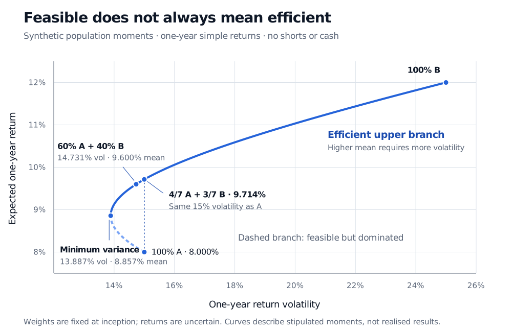
Hypothetical long-only two-asset mean–volatility curve. The minimum-variance portfolio has volatility 13.887% and expected return 8.857%. The upper branch to B at 25% volatility and 12% expected return is efficient. A alone has 15% volatility and 8% expected return; weights 4/7 in A and 3/7 in B have the same 15% volatility and 9.714% expected return.

Original synthetic example: stipulated one-year population moments, fully invested long-only weights, no cash or costs. The solid upper branch is efficient; the dashed lower branch contains attainable but dominated portfolios.

There is also an exact same-risk comparison. Investing

4/7

in A and

3/7

in B gives 15% volatility, equal to A alone, but an expected return of 9.7142857…% rather than 8%. The improvement is about 1.714 percentage points of expected return at the same modelled volatility. It is not a guaranteed extra profit next year.

Where the frontier begins—and why the lower branch is excluded

Complete the square in the variance formula:

\sigma_p^2(x)=\frac{27}{1400} +0.07\left(x-\frac{3}{14}\right)^2.

The global minimum-variance portfolio therefore holds

11/14

in A and

3/14

in B: approximately 78.571% / 21.429%. Its expected return is 8.8571429…%, variance is

27/1400

, and volatility is 13.8873015…%. This is the leftmost attainable point in the chart.

For $0\le x<3/14$ , moving toward that point raises expected return while lowering volatility. Every portfolio on this lower branch is dominated by the minimum-variance portfolio. Drawing the whole curved locus and calling it the efficient frontier would include choices the definition rules out.

For

3/14\le x\le1

, both expected return and volatility rise with

x

. No other allowed weight offers a higher mean without higher volatility, or lower volatility without a lower mean. This upper branch, including the minimum-variance endpoint, is the efficient frontier for this example. It ends at B alone because B has the highest expected return and leverage is prohibited.

With two assets and one budget constraint, the feasible combinations form this curve rather than a filled region. Larger asset universes generally produce a region of attainable risk–return pairs; the frontier is its nondominated boundary. Neither an individual asset nor an arbitrary diversified allocation automatically lies on it. Elton, Gruber, Brown and Goetzmann explain this distinction in Chapter 5 of Modern Portfolio Theory and Investment Analysis, ninth edition, especially pp. 76–78.

From a drawing to a constrained optimisation problem

For $n$ assets, collect expected returns in $\mu$ and covariances in $\Sigma$ . The basic quantities are

\mu_p=\mathbf w^\top\mu, \qquad \sigma_p^2=\mathbf w^\top\Sigma\mathbf w.

One way to construct the frontier through mean–variance optimisation is to vary a required expected return $m$ and solve

\begin{aligned} \min_{\mathbf w}\quad&\mathbf w^\top\Sigma\mathbf w\\ \text{subject to}\quad&\mathbf 1^\top\mathbf w=1,\\ &\mathbf w\ge0,\\ &\mathbf w^\top\mu\ge m. \end{aligned}

Here

m

is a minimum expected return, not a promised payout. In the two-asset example, a requirement below 8.8571429…% returns the same minimum-variance portfolio; raising it from that mean to 12% traces the upper branch. A requirement above 12% is infeasible. By contrast, forcing an equality to an 8% mean produces A alone, a minimum-variance solution at that exact mean which is nevertheless dominated. A solver label cannot replace the economic definition. If several variance-minimisers tie, retain the one with the highest mean before labelling a point efficient.

Constraints define the comparison. Add a maximum 40% weight in B, and the frontier ends at the 60/40 portfolio: 9.6% expected return and about 14.731% volatility. The minimum-variance allocation still satisfies that cap, but a 10% expected-return requirement becomes infeasible. Removing a constraint enlarges the feasible set under the same inputs; it may introduce portfolios that dominate previously efficient choices.

The fully-invested mean–variance derivation develops a closed-form alternative with a positive-definite covariance matrix and unrestricted signed weights. Its formulas cannot simply be applied unchanged to the long-only problem above. The full lesson requires membership; a public preview is available.

What the curve leaves unresolved

The inputs can move the boundary. In actual research, expected returns and covariances are estimated. An allocation that is efficient for those estimates may be poor for a nearby plausible set of inputs. Weight caps, covariance shrinkage and sensitivity analysis can help control that instability, but an attractive fitted curve is not evidence of future performance. Kim and Boyd's robust-frontier research explicitly treats uncertainty in those inputs.

Volatility is a chosen risk measure. Mean–variance efficiency does not establish superiority for investors who care about crash exposure, liquidity, maximum drawdown, liabilities or other features of the return distribution. Normality is unnecessary for the calculations; using two moments as a complete ranking of risky investments needs an additional preference or distributional justification.

Cash changes the problem. Adding a genuinely risk-free asset with a matched one-year return introduces new feasible combinations. Under suitable borrowing and lending assumptions, a line through the cash return can be tangent to the risky frontier. Different borrowing rates, leverage limits or a ban on borrowing change that construction. The risky-only curve here does not itself assert a capital market line or identify the market portfolio.

Sources

Harry Markowitz, “Portfolio Selection”, The Journal of Finance 7(1), 1952, pp. 77–91, especially pp. 79–82: portfolio moments and efficient expected-return/variance combinations. Original paper; the example and figure above are independently constructed.
Edwin J. Elton, Martin J. Gruber, Stephen J. Brown and William N. Goetzmann, Modern Portfolio Theory and Investment Analysis, 9th edition, Wiley, 2014, Chapter 5, especially pp. 76–78: the no-short-sales efficient frontier; pp. 81–85: riskless lending and borrowing.
Seung-Jean Kim and Stephen Boyd, Robust Efficient Frontier Analysis with a Separable Uncertainty Model, November 2007, §§1.1–1.2: constrained feasible sets, efficient-frontier construction and sensitivity to estimated inputs.

A portfolio can be feasible and still waste risk

Where the frontier begins—and why the lower branch is excluded

From a drawing to a constrained optimisation problem

What the curve leaves unresolved

Sources

Related terms

Correlation

Covariance

Diversification

Expected return

Maximum drawdown

Portfolio

Variance