Diversification reduces portfolio risk through imperfect co-movement. Derive the equal-weight risk floor and see why ten holdings are not ten independent risks.
Diversification
Diversification means spreading a portfolio across exposures whose outcomes do not move together perfectly, so that concentrating less on any one source of risk can reduce the risk of the whole. The important unit is the source of risk, not the number of lines on a holdings statement.
A fund can own many companies yet remain heavily exposed to one interest-rate shock, one commodity price or one customer base. Conversely, a small allocation to an exposure that behaves differently may change portfolio risk more than adding another similar stock. Markowitz's original Portfolio Selection paper, especially pp. 79–81 and 89, develops this distinction through covariance rather than security count.
Ten holdings, one shared problem
Imagine an investment committee splitting USD 100,000 equally among ten businesses: USD 10,000 in each. Company-specific product launches, lawsuits and operating problems differ, but all ten businesses remain exposed to weak aggregate demand. This is an original hypothetical example, not a claim about a particular market or sector.
Suppose each company's one-year simple total return has volatility 20%, and every distinct pair has correlation 0.25. Measure returns in the same currency, including distributions. Hold the beginning-of-year weights through the year, with no external cash flows, borrowing or trading costs. These are stipulated population moments; they are not estimates from a price sample.
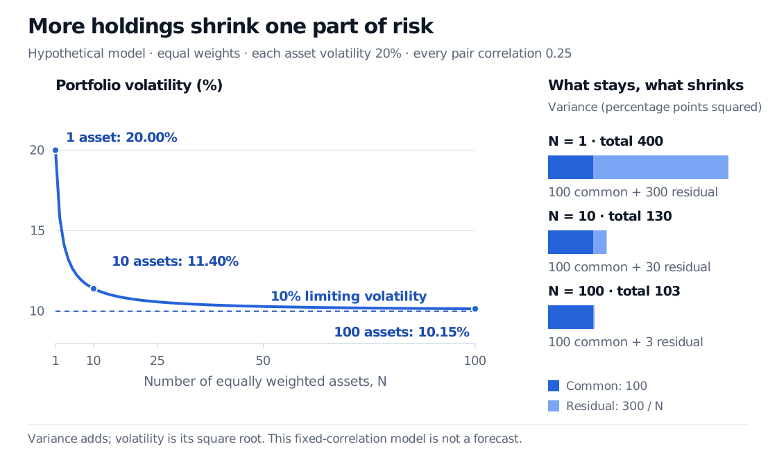
The ten-asset portfolio has volatility 11.40%. That is a substantial reduction from 20%, but far above the 6.32% obtained by incorrectly treating these returns as uncorrelated. The businesses share a risk that averaging cannot remove within this model.
Here is the calculation. If Ri is asset i's return and wi its fixed beginning weight, the portfolio return is Rp=∑i=1NwiRi. Its variance is
Var(Rp)=i=1∑Nwi2σi2+2i<j∑wiwjCov(Ri,Rj).
Covariance records whether deviations from the assets' respective means reinforce or offset each other. With fixed positive weights and unchanged individual variances, a lower covariance reduces portfolio variance, provided the resulting covariance matrix is valid. The sign qualification matters: for a long–short pair, the weight product is negative and the direction reverses.
For equal weights wi=1/N, equal individual volatility σ and equal pairwise correlation ρ, every off-diagonal covariance is ρσ2. There are N diagonal terms and N(N−1) ordered off-diagonal terms. Therefore
σp2=N2Nσ2+N(N−1)ρσ2=σ2(ρ+N1−ρ).
For the committee's ten businesses,
σp2=0.04(0.25+100.75)=0.013,σp=0.013≈11.40%.
The variance is 0.013 in decimal-return-squared units, or 130 percentage points squared. It is not a volatility of 1.3%. Variance and volatility have different units; take the square root before expressing the result as a return percentage.
No normal-distribution assumption is needed. These return and variance identities require the stated linear portfolio aggregation and finite second moments. They do not specify the probabilities of particular losses or make mean and variance a complete description of investment risk.
The part that does not average away
Rearranging the same result separates two components:
σp2=common componentσ2ρ+component reduced by averagingNσ2(1−ρ)=0.01+N0.03.
In this positive-correlation model, one representation gives every company the same common shock plus a company-specific shock uncorrelated with the common shock and the other company-specific shocks. The common variance is 0.01; the company-specific variance is 0.03 per company. Equal weighting averages the latter down, while every holding still carries the common shock. This is the mechanism illustrated by the figure, rather than a measured attribution of real company returns.
Portfolio volatility declines from 20% with one asset to 11.40% with ten and 10.15% with one hundred, approaching a 10% floor. Variance bars show common risk of 100 percentage points squared, plus residual risk of 300 divided by the number of assets.
Original hypothetical model: equal beginning weights, one-year simple returns, individual volatility 20% and every pairwise correlation 0.25. The curve shows volatility; the stacked bars show additive variance components.
Number of holdings
Portfolio variance, decimal-return squared
Portfolio volatility
1
0.0400
20.00%
2
0.0250
15.81%
10
0.0130
11.40%
100
0.0103
10.15%
Limit as N→∞
0.0100
10.00%
The first additions do much more than later ones. A hundred names come closer to the floor, but do not remove it. The 10% floor belongs to this specified universe and covariance structure. It is not a universal minimum achievable risk: changing exposures, introducing a different asset or constructing a hedge changes the problem.
At zero pairwise correlation, the formula becomes σp=σ/N. At correlation one, it becomes σp=σ: adding copies of the same return exposure provides no variance reduction. Negative correlations can be helpful, but a many-asset equal-correlation matrix must satisfy ρ≥−1/(N−1) for N>1. You cannot assume the same fixed negative correlation for arbitrarily many assets and still have a valid joint model.
A holdings list is only the start of the audit
The SEC's diversification guidance recommends looking both across and within asset classes, and checking overlapping holdings when owning several funds. Three funds that own the same large companies may repeat exposures. Sector labels alone also miss shared factor exposures, such as sensitivity to financing conditions.
Useful questions go beyond “how many names?”:
What dominates the weights and risk? A portfolio with one large holding and many tiny ones is not the equal-weight portfolio above. Adding a volatile asset can increase total variance even when its correlation is below one.
What happens under a different joint scenario? If the example's correlation rises from 0.25 to 0.75 while each volatility stays at 20%, ten-asset volatility rises to 17.61%. Real volatilities can change too. Correlations need not always rise in stress; the point is to test the joint exposure rather than freeze one estimate.
Can the portfolio survive the path? Common downside events, illiquid exits, margin calls and funding withdrawals can defeat a plan built only around ordinary-period variance. Leverage can amplify a smaller return fluctuation into a serious equity loss.
Lower variance does not imply that every loss becomes smaller, or that a loss cannot occur. Two portfolios can have equal variance and very different downside tails. Stress testing complements the covariance calculation by asking what specific shocks do to the whole book.
Diversification also does not manufacture expected return: for fixed beginning weights, expected portfolio return is the weighted average of the individual expected returns. Choosing exposures and deciding the trade-off between return, risk, costs and constraints leads to the efficient frontier, rather than a rule to buy the largest possible number of names.
Finally, weights drift when asset values change. Rebalancing can restore an intended allocation, but trading costs and taxes affect how to do it. ASIC's Moneysmart guide explains this distinction between building a mix and maintaining it, including the currency exposure introduced by overseas holdings.
For the probability foundations and a two-asset worked example, read Expectation, Variance and Covariance, available in full with a free signed-in account. For choosing weights subject to a budget and risk preferences, Mean–Variance Optimisation develops the matrix formulation; its full lesson requires membership.
Sources
Edwin J. Elton, Martin J. Gruber, Stephen J. Brown and William N. Goetzmann, Modern Portfolio Theory and Investment Analysis, 9th edition (2014), Chapter 4, pp. 56–58: equal-weight portfolio variance, average covariance and diversification limits. The financial story, numerical example and figure here are original.
Harry Markowitz, “Portfolio Selection”, The Journal of Finance 7(1), 1952, pp. 77–91, especially pp. 79–81 and 89: portfolio moments and diversification through covariance.