Calculate portfolio variance from weighted covariances, verify a 60/40 example with actual outcomes, and distinguish exact risk identities from estimated inputs.
Portfolio variance
Portfolio variance is the expected squared deviation of a portfolio's return from its expected return. It combines the uncertainty of each holding with the way the holdings move together. Its square root is portfolio volatility.
A manager cannot calculate it from position weights and individual volatilities alone. Two portfolios with identical holdings and standalone risk assumptions can have different total risk because their covariances differ.
For fixed weights collected in a column vector w and a return covariance matrix Σ,
σp2=Var(Rp)=w⊤Σw.
The transpose symbol turns the weight column into a row so that this matrix product produces a single number. What matters economically is the interaction it retains: each position's return is paired with every other position's return.
A 60/40 allocation with two sources of risk
Consider a hypothetical fund that puts 60% of its initial capital in sleeve A and 40% in sleeve B. It holds these positions for one year, without external cash flows or interim trading. Returns include distributions on a consistent reinvestment basis and use one reporting currency. Assume the following population moments, rather than estimates from a historical sample:
One-year simple-return input
Sleeve A
Sleeve B
Expected return
8%
12%
Volatility
15%
25%
Weight at the start
60%
40%
The correlation is ρAB=0.2. Correlation is dimensionless; covariance restores the return scale:
Cov(RA,RB)=ρABσAσB=0.2(0.15)(0.25)=0.0075.
The covariance matrix, using decimal returns, is
Σ=(0.02250.00750.00750.0625).
Its diagonal holds variances, so the 15% input enters as 0.152=0.0225. Substituting correlation 0.2 directly into the off-diagonal cells would mix different units and produce an invalid risk calculation.
Portfolio return is Rp=0.6RA+0.4RB. Its mean is 0.6(8%)+0.4(12%)=9.6%. Its variance requires squared weights and covariance:
Therefore σp=0.0217≈0.147309, or 14.73% over one year. The weighted average of the individual volatilities is 19%; it is the portfolio volatility only at perfect positive correlation for these positive weights. Here, diversification brings total volatility below even A's 15%, despite the allocation to the more volatile sleeve B. That is a result for these inputs, not a promise about every mixed portfolio.
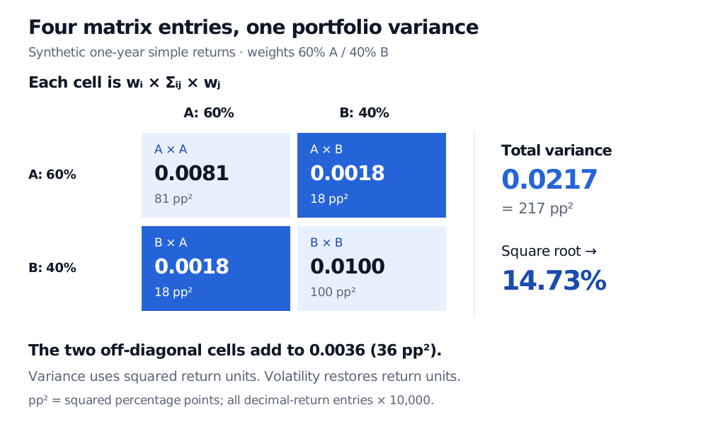
Weighted covariance ledger: the A diagonal contributes 0.0081, the B diagonal 0.0100, and the two off-diagonal entries contribute 0.0018 each. Total variance is 0.0217, or 217 squared percentage points, giving volatility 14.73%.
Each cell is a weighted covariance contribution, not a raw covariance-matrix entry. Original synthetic one-year example; decimal-return variance and squared-percentage-point units are shown together.
Read the units before reading the number. Variance 0.0217 is in squared decimal-return units; it is not a 2.17% volatility. If returns are entered as 15 and 25 percentage points instead of 0.15 and 0.25, variance is 10,000(0.0217)=217 squared percentage points. Its square root is 14.73 percentage points. The economic risk is identical under either consistent convention.
Why covariance appears twice
Let X=RA−E[RA] and Y=RB−E[RB]. Squaring the portfolio's deviation gives
(wAX+wBY)2=wA2X2+wAwBXY+wBwAYX+wB2Y2.
Taking expectations turns the squared deviations into variances and each product into covariance. The two cross terms are equal. This is why the two-asset formula contains 2wAwBCov(RA,RB).
With many assets, either count every ordered pair once, or count each distinct pair once and multiply it by two:
A covariance model should agree with the variance of the portfolio returns it generates. Build two independent factors U and V, each equally likely to be +1 or −1, and define
RA=0.08+0.15U,RB=0.12+0.05U+0.06V.
There are four equally likely joint states. A depends on the common factor U; B has a smaller loading on U plus its own independent factor V.
U
V
A return
B return
60/40 portfolio return
+1
+1
23%
41.4949%
30.3980%
+1
−1
23%
−7.4949%
10.8020%
−1
+1
−7%
31.4949%
8.3980%
−1
−1
−7%
−17.4949%
−11.1980%
Original hypothetical distribution, not historical observations; displayed outcomes are rounded.
Both factors have mean zero and variance one. Consequently A's variance is 0.0225, B's is 0.052+0.06=0.0625, and their covariance is 0.15(0.05)=0.0075.
More directly, the portfolio return simplifies to
Rp=0.096+0.11U+0.40.06V.
Its centered squared outcomes average to
41s=1∑4(Rp,s−0.096)2=0.112+0.42(0.06)=0.0217.
This independently reproduces the matrix answer. No normal distribution was needed. Fixed linear exposures and finite second moments suffice for the variance identity. A variance alone, however, does not determine a loss probability or value at risk; those require additional information about the distribution.
What changing correlation really changes
Keeping these weights and individual volatilities fixed gives
σp2=0.0181+0.018ρAB.
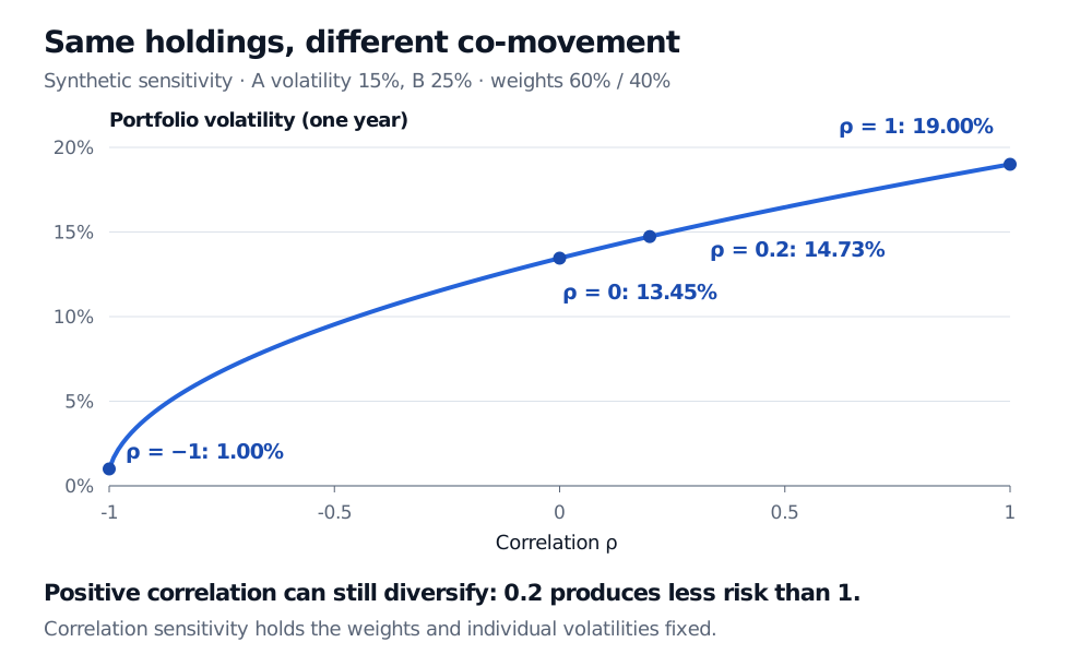
At correlation zero, volatility is about 13.45%. At correlation one, it is 19%. At correlation minus one, it is 1%: the weighted volatility exposures, 9% and 10%, nearly offset but do not cancel completely.
Fixed 60/40 portfolio sensitivity to correlation: volatility rises from 1.00% at correlation minus one to 13.45% at zero, 14.73% at 0.2, and 19.00% at one. Individual one-year volatilities remain 15% and 25%.
Original synthetic sensitivity. Weights and individual one-year volatilities stay fixed; only correlation changes.
Negative correlation is therefore unnecessary for a diversification benefit relative to perfect positive correlation. But the direction depends on the exposure signs: with one long and one short position, wAwB<0, so higher covariance reduces this pair's variance, holding everything else fixed. Shorting also introduces financing, borrowing and liquidity considerations outside this covariance calculation.
From a clean identity to a credible risk number
The formula is exact for the stated model. Whether its inputs describe the portfolio is a separate question.
Align the return definition and horizon. Use common observation dates, currency treatment and price-versus-total-return conventions. The one-year inputs above need no annualisation. Multiplying a daily covariance matrix by a trading-day count concerns sums of daily returns under dependence assumptions; it does not generally give the exact covariance of compounded annual simple returns.
Separate a population from an estimate. For T aligned observations, the usual sample matrix has entries Σij=T−11∑t=1T(Ri,t−Rˉi)(Rj,t−Rˉj). With the same rows, centering, divisor and fixed weights, w⊤Σw equals the sample variance of the weighted return series. The four states above describe an entire stipulated probability distribution, so their population calculation divides by four. Historical estimates remain uncertain forecasts of future co-movement.
Require a coherent matrix. A covariance matrix is symmetric and positive semidefinite: x⊤Σx≥0 for every real exposure vector x. Estimating different pairs on different date sets can violate that requirement. Valid pairwise correlations alone do not guarantee a valid many-asset matrix. A singular matrix can still calculate variance; inversion is unnecessary here.
Match the exposure model to the holdings. Beginning-of-period wealth weights give the simple-return identity for the held portfolio. Log returns do not aggregate this way. Rebalancing requires a return calculation for each holding period. Signed exposures can instead be measured relative to stated reference capital, with financing included explicitly. For options and other nonlinear positions, full revaluation or a justified local risk approximation is needed before using underlying-factor covariances.
Variance treats upside and downside deviations alike. It is useful for comparing spread around a mean, but cannot by itself describe tail shape, funding pressure or the probability of a damaging drawdown. Choosing weights using expected return and this risk measure belongs to mean–variance optimisation; calculating variance for the weights already held is the step developed here.
For a worked introduction to the underlying moments, read Expectation, Variance and Covariance (full lesson free with a signed-in account; public preview available). The Mean–Variance Optimisation lesson develops portfolio choice and benchmark-relative risk (membership for the full lesson; public preview available).
Sources
Elton, E. J., Gruber, M. J., Brown, S. J. and Goetzmann, W. N., Modern Portfolio Theory and Investment Analysis, 9th edition, Chapter 4, “Characteristics of Portfolios in General,” pp. 50–54: portfolio-return aggregation, two-asset variance and covariance, and direct outcome verification.
Eric Zivot, University of Washington, Portfolio Theory with Matrix Algebra, Spring 2015, slides 6–10: return and covariance-matrix notation. The slides also impose a normal-return model; the variance identity used here follows without that assumption, as the discrete construction demonstrates.