Calculate covariance from paired returns, distinguish sample and population divisors, track squared units, and see exactly how co-movement changes portfolio risk.
Covariance
Covariance measures whether two quantities tend to lie on the same side of their own averages or on opposite sides. In portfolio risk, it captures how the returns of two holdings combine: individual risks do not simply add, because the holdings can amplify or offset one another's fluctuations.
For two random variables X and Y with finite variances and means μX=E[X] and μY=E[Y],
Cov(X,Y)=E[(X−μX)(Y−μY)].
The expected value averages a product of deviations, not a product of raw levels. A positive product occurs when both quantities are above their means or both are below. A negative product occurs when one is above and the other below. Covariance averages their sizes as well as their signs; it does not count how often prices rise together.
Four paired returns, calculated by hand
Suppose a researcher has four synthetic observations of two strategies' simple returns. Each row covers the same period, on the same return and currency basis. These are illustrative data, not a historical backtest. The arithmetic mean return is 1% for A and 0.5% for B.
Period
A return
B return
A deviation (pp)
B deviation (pp)
Product (pp²)
1
2%
1%
1
0.5
0.5
2
−1%
2%
−2
1.5
−3
3
3%
−1%
2
−1.5
−3
4
0%
0%
−1
−0.5
0.5
Sum
0
0
−5
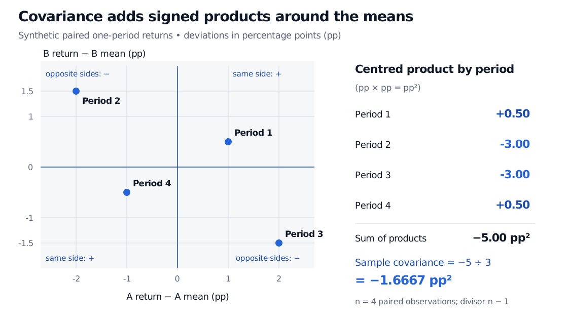
Here pp means percentage points. Period 4 contributes positively even though neither strategy earns a positive return: both are below their own sample means. Periods 2 and 3 supply the larger negative products.
To estimate population covariance from n≥2 paired observations, the usual sample estimator is
Four synthetic paired-return deviations. Periods 1 and 4 contribute plus 0.5 percentage-point squared each; periods 2 and 3 contribute minus 3 each. The sum is minus 5 and the sample covariance is minus 1.6667 percentage-point squared.
Original synthetic four-period example. Both axes measure deviations from sample means in percentage points; signed products have units pp². Sample divisor: n−1=3.
Why the divisor and units matter
The n−1 correction compensates for estimating the means from the same observations. It makes sample covariance unbiased under independent, identically distributed paired draws with finite second moments. It does not make four observations a reliable forecast, and that sampling argument should not be assumed for a serially dependent financial time series.
If the four rows instead describe the entire stipulated population, each with probability 1/4, average the products with divisor four. That model's covariance is −5/4=−1.25 pp², or −0.000125 in decimal-return squared. Both calculations are legitimate; they answer different questions.
A 2% return is 0.02 in decimal form and 2 in percentage-point units. Converting both return series from decimals to percentage points multiplies covariance by 100×100=10,000. The numerical value −1.6667 is therefore not “−166.67% covariance,” and it is not a correlation. Always retain the unit convention.
Covariance supplies the missing portfolio term
Consider a portfolio allocated 50% to each strategy at the start of each observation period. Assume no fees or external cash flows. Its one-period simple return is Rp=0.5A+0.5B. These fixed weights mean rebalancing between periods if needed; they are not the drifting weights of an unrebalanced buy-and-hold portfolio.
The identity also holds for sample moments calculated on the same rows with the same divisor. Here the individual sample variances are sA2=1/3000 and sB2=1/6000 in decimal-return squared. Hence
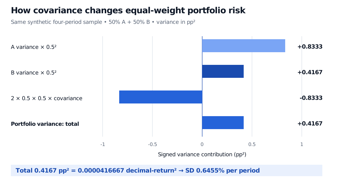
The standard deviation is 1/24000≈0.006455, or 0.6455% per observation period. An independent check is to calculate the portfolio returns directly: 1.5%, 0.5%, 1% and 0%, with mean 0.75%. Their sample variance gives exactly the same answer.
Equal-weight portfolio variance contributions in percentage-point squared: A contributes plus 0.8333, B plus 0.4167, and the covariance cross term minus 0.8333, leaving total 0.4167 and standard deviation 0.6455% per period.
Original synthetic sample, same four paired periods. Signed contributions add to portfolio variance; standard deviation is the square root of the total, not the sum of separate square roots.
This is the mechanism behind diversification. For fixed positive weights and individual variances, lower covariance reduces portfolio variance. Positive covariance can still permit a diversification benefit; it need not become negative. With one position short, wAwB is negative, so the direction reverses: higher covariance can improve the offset between the two exposures.
Scale, correlation and the covariance matrix
Covariance carries the product of its inputs' units. For dollar profit and loss, it is dollar-squared; for two decimal returns, it is decimal-return squared. Increasing position size changes dollar covariance even if the underlying relationship is unchanged.
For constants a,b,c,d,
Cov(aX+b,cY+d)=acCov(X,Y).
Adding a constant shifts a mean but leaves the deviations unchanged. Multiplying an exposure scales its covariance; reversing its sign reverses the covariance's sign. Also, Cov(X,X)=Var(X), and a constant variable has zero covariance with every variable of finite variance.
Correlation removes scale by dividing by the two standard deviations:
Unlike covariance, correlation lies between −1 and 1. If either standard deviation is zero, correlation is undefined even though covariance is zero. More generally, ∣Cov(X,Y)∣≤σXσY; covariance has a scale-dependent bound, not a universal bound of one.
For many holdings, a covariance matrix collects individual variances on the diagonal and pairwise covariances off the diagonal. The two-strategy sample matrix is
S=(1/3000−1/6000−1/60001/6000).
Then portfolio variance is wTSw. A covariance matrix must produce a nonnegative variance for every weight vector. Estimating different entries from incompatible dates or independently altering them can break that consistency.
What a covariance estimate cannot tell you
Zero covariance does not establish independence. For example, let a synthetic market shock X take −2%, 0% and 2% with equal probabilities, and let Y=X2. Symmetry makes E[X]=E[X3]=0, so Cov(X,Y)=0. Yet knowing X determines Y exactly. Here Y is squared return, a measure of shock magnitude, rather than another asset return. Nonlinear exposures can have a substantial relationship that signed linear co-movement misses.
An estimate also depends on the data window and observation clock. Align timestamps before pairing returns; stale prices, missing observations, mixed currencies and overlapping horizons change what is measured. A negative covariance in this four-row example supplies no evidence that the strategies will hedge one another in a future crisis. The basic covariance alone describes neither tail dependence nor causal direction.
For a guided foundation, Expectation, Variance and Covariance develops the probability definition and two-asset risk formula. Its public page is a preview; the full Mathematics Primer lesson is available with a free signed-in account.
Practice
1. Three synthetic paired periods give A returns of 0%, 2%, 4% and B returns of 3%, 1%, 2%, respectively. Calculate sample covariance in pp² and decimal-return squared. What changes if these are three equally likely states of the entire model population?
Answer. Both means are 2%. The centred products in pp² are (−2)(1)=−2, (0)(−1)=0, and (2)(0)=0. Sample covariance is −2/(3−1)=−1 pp², or −0.0001 decimal-return squared. For the stipulated population use divisor three: −2/3 pp², or approximately −0.000066667. Switching divisor changes the estimand; changing units changes the numerical scale.
2. A desk holds a long exposure of 1 to X and a short exposure of 0.5 to Y, both measured relative to the same reference capital. One-period return volatilities are 10% and 20%, and covariance is 0.01 in decimal-return squared. What is the exposure's standard deviation? Would replacing covariance with zero reduce it?
Answer. The P&L per unit of reference capital is X−0.5Y, so its variance is 0.102+(−0.5)2(0.202)+2(1)(−0.5)(0.01)=0.01. Its standard deviation is 10%. At zero covariance the variance would be 0.02 and standard deviation approximately 14.14%. Positive covariance helps these long and short exposures offset. The weights are exposures on reference capital, not fully invested long-only allocation weights.
Sources
Dimitri P. Bertsekas and John N. Tsitsiklis, Introduction to Probability, 2nd edition (2008), §4.2, pp. 218–222: population covariance, correlation, linearity, independence and variance of sums. The return fixtures, figures and practice questions above are original.