Pearson correlation measures linear co-movement on a unit-free scale. Calculate paired-return correlation, understand its sign and see why zero correlation can hide dependence.
Correlation
Correlation measures the direction and strength of linear co-movement between two quantities. Unless another measure is named, finance usually means Pearson correlation: covariance divided by the two standard deviations. Its unit-free scale makes the co-movement of two daily return series comparable even when their volatilities differ.
For a portfolio manager, this answers a specific question: when one return is above its own average, does the other tend to be above or below its own average? It does not tell you whether both investments are profitable, whether one causes the other, or whether they can lose together in a crisis.
The denominator makes the comparison portable
For random variables X and Y with finite, strictly positive variances, population correlation is
ρXY=σXσYCov(X,Y),σX=Var(X),σY=Var(Y).
Covariance records the average product of deviations from expected values. Dividing by the standard deviations removes the units and puts the result between −1 and 1:
Positive correlation: deviations in the same direction dominate the covariance calculation.
Negative correlation: deviations in opposite directions dominate.
Zero correlation: those products average to zero; this need not mean there is no relationship.
The endpoints are exact statements. Correlation +1 requires Y=a+bX with b>0, with probability one; correlation −1 requires the same affine relation with b<0. A large absolute correlation is not the same thing as a steep slope. A change of units can make a slope much steeper while leaving correlation unchanged.
More precisely, for nonzero constants a,c,
Corr(aX+b,cY+d)=sgn(ac)ρXY.
Writing both returns as percentages instead of decimals multiplies each by 100, so correlation stays the same. Reversing the sign of one quantity flips correlation's sign. Thus an exposure to −Y has the opposite correlation with X; an actual short position's return also depends on its financing, costs and chosen capital denominator. If either variable is constant, its standard deviation is zero and Pearson correlation is undefined, not zero.
Four observations, one estimate
Suppose a researcher checks two hypothetical strategies over four identical holding periods. These are simple returns, measured on the same dates and basis, with no annualisation:
Period
Strategy A
Strategy B
1
2%
1%
2
−1%
2%
3
3%
−1%
4
0%
0%
The sample means are Aˉ=0.01 and Bˉ=0.005. For n matched pairs, sample Pearson correlation is
Using decimal returns, the centred cross-product sum is −0.0005, while the two centred squared sums are 0.001 and 0.0005. Hence
r=0.0010.0005−0.0005=−21≈−0.7071.
Equivalently, divide all three sums by n−1=3: sample covariance is −1/6000, and sample variances are 1/3000 and 1/6000, all in decimal-return-squared units. Their standard deviations are about 1.8257% and 1.2910% per observed period. The common divisor cancels in correlation. Using n consistently in all three quantities would give the same r; mixing divisors would not.
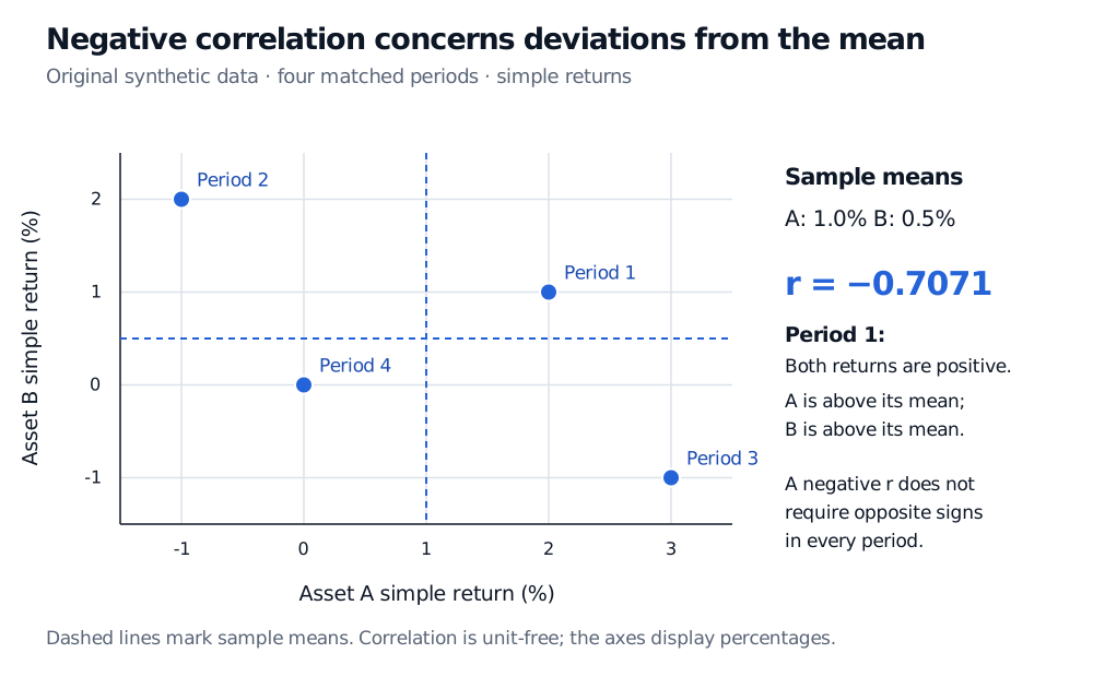
Four synthetic paired returns: A is 2, −1, 3 and 0 percent; B is 1, 2, −1 and 0 percent. Dashed sample means are 1 percent for A and 0.5 percent for B. Sample correlation is −0.7071, although both returns are positive in period 1.
Original synthetic four-period sample. Dashed lines mark sample means; all axes display simple returns in percent.
The negative estimate does not mean B loses whenever A gains. In period 1 both gain and both are above their own means. Period 4 has two zero returns, but both are below their respective positive means. Correlation aggregates centred products across the entire sample; it is neither a count of opposite-sign returns nor a probability that a hedge succeeds.
The formula computes a descriptive statistic without requiring normally distributed returns. Treating it as an estimate of a stable population parameter requires a defensible sampling model. Four observations make the arithmetic visible; they do not establish a reliable hedge relationship. The n−1 correction makes sample covariance unbiased under i.i.d. paired sampling with finite second moments. It does not make the ratio r exactly unbiased for ρ.
Why a risk desk needs more than the coefficient
For a two-asset portfolio with fixed weights and matched-period returns,
Var(Rp)=wA2σA2+wB2σB2+2wAwBρABσAσB.
For two positive weights and fixed individual volatilities, lower correlation reduces variance: this is the co-movement mechanism behind diversification. With one negative weight, the cross-term changes sign. Correlation alone therefore cannot rank portfolio risk without the exposures and volatilities. Even an exact low variance says little about the particular losses that matter unless the rest of the return distribution is understood.
A practical estimate also needs its question written beside it:
Returns or levels? Two price levels can trend together and produce a high coefficient without a dependable relationship between their returns. A level correlation is not evidence that their spread will revert. Simple and log returns can also give different estimates; choose the convention for the task.
Which pairs? Match currencies, adjustment conventions, return horizons and timestamps. Different market closing times can distort contemporaneous correlation. Missing observations are not zero returns.
Which window? An estimate over one historical period need not describe the next regime. Compare windows and stress scenarios rather than treating an estimated coefficient as a contractual hedge ratio.
Which dependence? A scatter plot can reveal curvature, unusual observations or separate clusters that one coefficient hides. Correlation is sensitive to extreme observations; removing them merely to improve the coefficient can remove the very losses a risk model should examine.
Neither a coefficient nor a scatter plot establishes causation. Both strategies might respond to the same market shock. NIST's scatter-plot guidance separates linear and nonlinear patterns from causal claims.
A relationship that correlation cannot see
Consider an exact model distribution: X takes −1,0,1 with equal probabilities, and Y=X2. Then
E[X]=0,E[Y]=32,E[XY]=E[X3]=0.
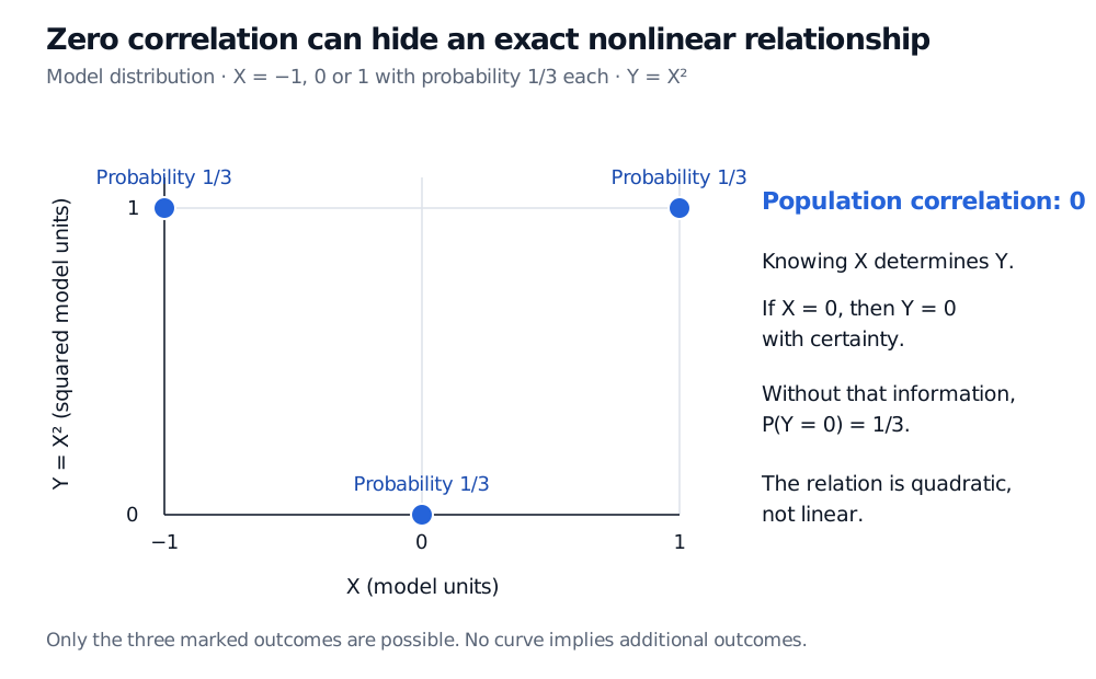
Consequently Cov(X,Y)=0. Both variances are positive—Var(X)=2/3 and Var(Y)=2/9—so correlation exists and equals zero. Nevertheless, X determines Y completely:
P(Y=0∣X=0)=1,P(Y=0)=31.
The exact model has outcomes (−1,1), (0,0) and (1,1), each with probability one third. Population correlation is zero, but knowing X determines Y because Y equals X squared.
Exact discrete model, not sampled market data. Only the three marked outcomes are possible; the dependence is quadratic.
This shows why independence implies zero correlation when the requisite moments exist, while zero correlation generally fails to imply independence. In finance, a quantity linked to the magnitude of a market move can have little linear correlation with its signed return. Nonlinear payoffs and joint extreme losses need their own analysis. Under the stronger assumption that the pair is jointly normal, zero correlation does imply independence; normal marginal distributions alone are insufficient.
For a short foundation with portfolio calculations, read Expectation, Variance and Covariance, available in full with a free signed-in account. The deeper Covariance and Correlation lesson develops the population identities and perfect-correlation cases; its full text requires membership, with a public preview.
Practice: audit a small return sample
Three matched periods give A returns of −1%, 0%, 1% and B returns of 2%, 0%, 1%. Compute sample correlation using n−1 sample moments. Does expressing returns as percentages change it? What happens if B's numerical exposure is negated?
Answer. In decimals, the means are Aˉ=0 and Bˉ=0.01. The deviations are (−0.01,0,0.01) and (0.01,−0.01,0). Their cross-product sum is −0.0001 and each squared-deviation sum is 0.0002. Dividing by two gives sample covariance −0.00005 and each sample variance 0.0001. Therefore
r=0.00010.0001−0.00005=−0.5.
Percentage display leaves r=−0.5 unchanged; negating B gives +0.5. The coefficient describes these three pairs. It does not establish a population correlation or guarantee future loss protection.
Sources
Dimitri P. Bertsekas and John N. Tsitsiklis, Introduction to Probability, 2nd edition (2008), §4.2, especially pp. 219–222: population correlation, its bounds, affine endpoints and the distinction between uncorrelated and independent variables. The data, nonlinear model presentation, figures and practice calculation here are original.
NIST Dataplot: Correlation, equation 2-5 — the centred sample Pearson formula and its linear interpretation.