Fit a market-return exposure line, read residuals and R-squared, track return units, and separate sample fit from inference, causality and forecasting.
Linear regression
Linear regression describes a numerical response using a weighted sum of explanatory variables and an intercept. In its simplest form, it fits a straight line to paired observations. A quant might regress a fund's weekly excess return on the market's weekly excess return to estimate its market exposure, or relate tomorrow's return to information available today to build a forecasting model. These are different research questions, even when the fitted equations look similar.
Ordinary least squares, or OLS, is a common way to estimate a linear regression: choose the coefficients that minimise the sum of squared vertical differences between observed and fitted responses. Other estimators exist; the regression model and its estimation method are separate choices. NIST's least-squares treatment gives the corresponding objective and coefficient formulas.
What the line actually estimates
For one explanatory variable, write a population model as
Yi=a+bXi+εi.
The intercept a is the model's response at X=0; the slope b measures response units per explanatory-variable unit. The error εi captures what the line leaves out. If Eεi∣Xi]=0, then a+bXi is the [conditional expectation of Yi. Without that condition, a best linear approximation can still be useful, but it need not describe the conditional mean correctly at every X.
The fitted line from a finite sample is y^i=a^+b^xi. A residual is ei=yi−y^i: an observed discrepancy calculated after fitting. It is distinct from the unobserved population error. OLS solves
a,bmini=1∑n(yi−a−bxi)2.
With an intercept and nonconstant x values, the solution is
Here sxy is sample covariance, and sx2 is sample variance, both using the same divisor. The line passes through the two sample means. If every x is identical, the denominator is zero: the data cannot separate a slope from an intercept.
Five weeks, and a tempting performance claim
Suppose a researcher receives these synthetic weekly simple excess returns for a fund and market. Both subtract the same week's matched cash return. All table entries are percentages; residuals are percentage-point differences.
Week
Market excess return
Fund excess return
Fitted fund return
Residual, pp
1
−2.00%
−1.50%
−1.52%
+0.02
2
−1.00%
−0.50%
−0.56%
+0.06
3
0.00%
+0.20%
+0.40%
−0.20
4
+1.00%
+1.50%
+1.36%
+0.14
5
+2.00%
+2.30%
+2.32%
−0.02
Using decimal returns, xˉ=0, yˉ=0.004, the centred squared-x sum is 0.001, and the centred cross-product sum is 0.00096. Therefore
b^=0.96,a^=0.004,y^=0.004+0.96x.
The slope is an estimated market beta: a one-percentage-point difference in weekly market excess return corresponds to a 0.96-percentage-point difference in the fitted fund excess return. It does not mean a 1% proportional increase in the market's return produces a 96% proportional increase in the fund's return.
The intercept is 0.40% per week, the fitted excess return at a zero market excess return. In a market-factor regression this is a sample alpha. Five constructed rows cannot establish manager skill, persistent abnormal performance, or an annual return. Nor does estimating beta and alpha establish the CAPM expected-return restriction.
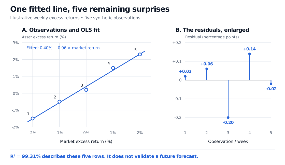
At a market excess return of 1%, the line gives 0.004+0.96(0.01)=0.0136, or 1.36%. Week 4 actually delivered 1.50%, leaving a positive 0.14-percentage-point residual. Week 3's negative residual says the fund fell short of its fitted value, despite having a positive excess return.
Five synthetic weekly market and fund excess returns with a fitted intercept of 0.40% per week and slope 0.96. A second panel enlarges residuals of +0.02, +0.06, −0.20, +0.14 and −0.02 percentage points. The in-sample R-squared is 99.31%.
Original synthetic weekly example. The first panel shows the fit; the second uses a different vertical scale to expose the remaining discrepancies. Neither panel shows future observations.
If both series are converted from decimals to percentages, the equation becomes y^%=0.40+0.96x%. The slope stays 0.96 because both axes change by the same factor. The intercept and residuals multiply by 100; their squares multiply by 10,000. Changing only one variable's units changes the slope too.
Why a near-perfect fit is not a forecast
For these observations, the residual sum of squares is RSS=0.0000064 in squared decimal-return units. The total centred response sum of squares is TSS=0.000928, so
R2=1−TSSRSS=145144≈0.9931.
The line accounts for approximately 99.31% of the fund's centred variation in this sample. That is not a probability of a correct prediction. With an intercept, nonconstant response and ordinary in-sample OLS, R2 lies between zero and one; the centred ratio is undefined for a constant response. The usual bounds need not hold for a test-set score or a fit without an intercept.
The market and fund observations here cover the same weeks. This is a contemporaneous exposure fit. At the start of next week, next week's market return is unknown; inserting its eventual value would not create a forecast available at the time of trading. A forecasting study must specify the target horizon, use only inputs already observable at the decision time, and evaluate later outcomes without refitting on them. That guards against look-ahead bias.
More explanatory variables, interactions or polynomial terms can reduce training RSS while worsening future errors: overfitting. Compare models on a later, genuinely held-out period using a sensible baseline and the same target. A causal claim needs a credible identification design addressing shared causes and other confounding; neither a slope nor a high R2 supplies that design.
Fitting is arithmetic; inference needs assumptions
OLS coefficients require data and a well-defined optimisation problem. They do not require normally distributed returns. Claims about uncertainty require more structure.
For the classical conditional linear model, take E[ε∣X]=0 and Var(ε∣X)=σ2I, with full-rank design. These conditions give unbiased coefficients and the usual covariance formula. Conditionally independent normal errors additionally give exact finite-sample t inference. In simple regression the classical estimated slope standard error is
SE(b^)=∑i(xi−xˉ)2RSS/(n−2).
The n−2 divisor allows for estimating two coefficients. In the example it gives approximately 0.04619 for the slope standard error, if the classical model applies. This arithmetic does not validate those assumptions in five synthetic weeks.
Financial residuals can have changing variance, serial dependence and influential extreme observations. Inspect residuals against fitted values and explanatory variables, and in time order; examine unusual points rather than deleting them merely because they hurt the fit. Heteroskedasticity-consistent or dependence-aware standard errors can address particular covariance failures under suitable conditions. They do not repair omitted-variable bias, a wrong conditional mean or unstable economic relationships. NIST's validation guidance explains why a single fit statistic cannot replace residual analysis.
Finally, linear means linear in the coefficients. A model containing x, x2 and an intercept is still linear regression, even though its fitted curve bends. Multiple regression adds explanatory variables, and each coefficient describes an association holding the included others fixed; highly correlated predictors can make individual coefficients imprecise. NIST illustrates this distinction.
To work through the essentials, read Basic Statistics and Regression, available in full with a free signed-in account. For the derivation, projection geometry and a slope confidence interval, continue to Linear Regression; its full text requires membership, with a public preview.
Sources
Gareth James, Daniela Witten, Trevor Hastie and Robert Tibshirani, An Introduction to Statistical Learning with Applications in R, 2nd edition (2021), §3.1.1–3.1.3 (least squares, coefficient uncertainty and model accuracy), §3.3.2–3.3.3 (extensions and potential problems). The authors' book site provides the text. The numerical example and figure here are original.