Market beta measures return sensitivity to a specified market benchmark. Calculate a sample beta, separate market exposure from total volatility, and combine signed portfolio exposures.
Market beta
Market beta measures the sensitivity of an asset’s return to a specified market return. It is the asset–market covariance divided by the market’s variance. Portfolio managers use it to describe, combine and hedge market exposure. It measures one source of co-movement; a low beta can coexist with large losses and high total volatility.
Specify the benchmark before quoting the number. A fund’s beta against a domestic equity index answers a different question from its beta against a global equity index. Neither index is automatically the all-asset market portfolio in economic theory.
The slope, with the return clock attached
Use matched-period simple excess returns
xt=RM,t−Rf,t,yt=Ri,t−Rf,t,
where both total returns include distributions, use the same currency and cover the same interval; Rf,t is the matched-period cash return. With finite second moments and positive market-excess-return variance, define
βi=Var(x)Cov(y,x).
This is the slope in the population best linear projection y=αi+βix+εi, whose residual has mean zero and zero covariance with x. A best linear projection exists without assuming normal returns or a linear conditional mean. Interpreting the line as the full conditional expectation requires an additional assumption.
The common divisor cancels if sample covariance and variance both use n−1. Do not mix divisors or fit through the origin by default: forcing a zero intercept generally changes the slope. If market variance is zero, beta is undefined.
Beta is dimensionless when both return series use the same units. A beta of 1.5 means that a one-percentage-point change in market excess return corresponds to a 1.5-percentage-point change along the fitted line. The intercept and residual still matter for the level of the asset’s return. Positive beta does not imply positive returns, and negative beta does not guarantee a gain in every market fall.
Some providers estimate beta using raw returns. If the cash return is constant across observations, subtracting it from both series leaves the slope unchanged. With time-varying cash returns the two slopes need not agree. Declare the convention.
Five weeks from a hypothetical fund
A risk analyst has five matched weekly observations. These are synthetic simple excess returns, displayed as percentages:
Week
Market
Fund
1
−2.00%
−1.50%
2
−1.00%
−0.50%
3
0.00%
0.20%
4
1.00%
1.50%
5
2.00%
2.30%
In decimal units, the market mean is zero and the fund mean is 0.004. The centred market squared sum is 0.001 and the centred cross-product sum is 0.00096. Therefore
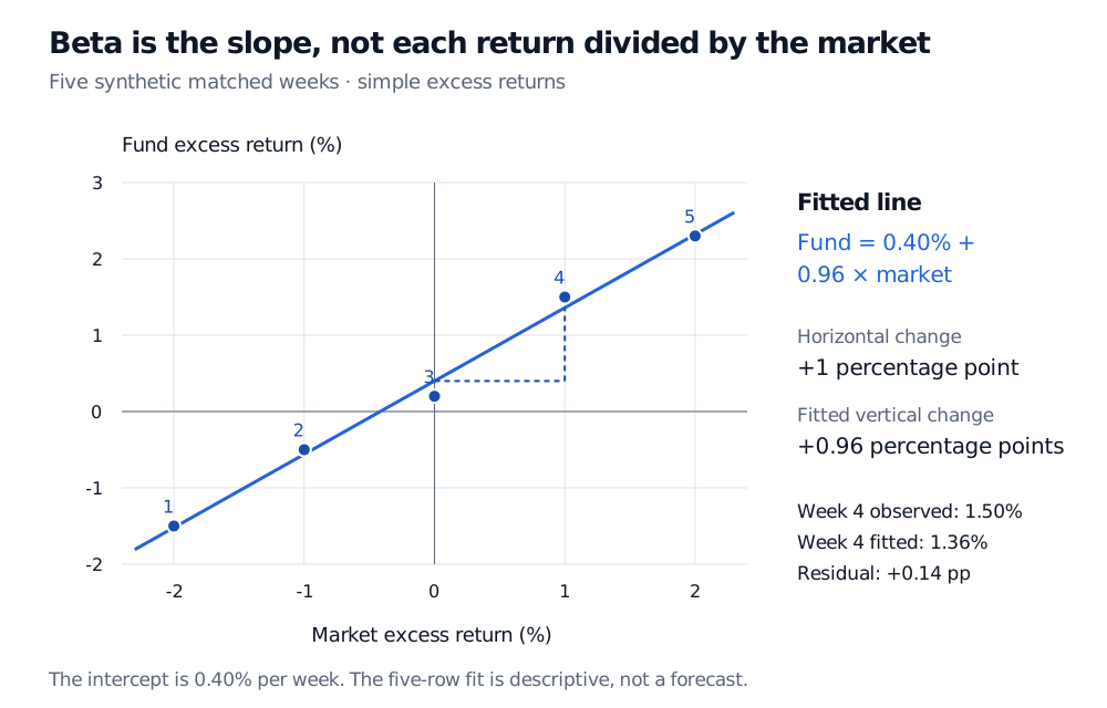
The fitted line is y^=0.004+0.96x. At market excess return 1%, the fitted fund excess return is 1.36%. The observed fund return that week was 1.50%, leaving a 0.14-percentage-point residual. The beta describes the slope of the fitted relationship, rather than each observed fund return divided by its market return.
Five synthetic weekly paired excess returns with fitted intercept 0.40% and slope 0.96; a one-percentage-point market change gives a 0.96-percentage-point fitted fund change.
Original synthetic weekly simple excess returns. Beta is the slope; individual points include residuals. Five rows do not establish a stable future exposure.
The intercept is an estimated weekly alpha relative to this benchmark and specification. Five illustrative weeks provide no evidence of persistent manager skill. This is also the paired-return example used in the linear-regression explanation, viewed here as a market-exposure calculation.
Why beta and volatility can tell different stories
For nonzero standard deviations,
βi=ρiMσMσi.
Here the volatilities and correlation refer to the same excess returns. Correlation measures standardised linear association and lies between −1 and 1. Beta also incorporates relative volatility, so its magnitude can exceed 1.
The projection gives the variance identity
σi2=βi2σM2+σεi2.
The market-related volatility is ∣βi∣σM; the sign of beta supplies the exposure direction. Add the variances, not the two volatilities. Residual risk is whatever this market projection leaves unexplained. It can include industry or other common factors, so calling all of it independent firm-specific noise would require more assumptions.
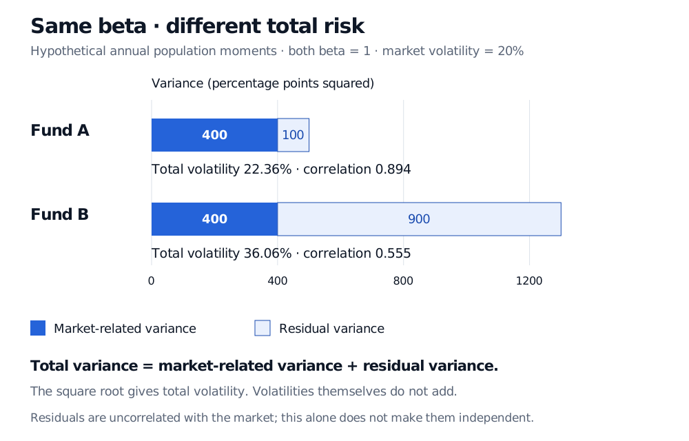
For example, stipulate annual market volatility of 20%. Two funds both have beta 1. Fund A has residual volatility 10%; Fund B has residual volatility 30%. Their total volatilities are respectively 22.36% and 36.06%, while their market correlations are approximately 0.894 and 0.555. The more volatile fund has the same beta and lower correlation.
Two hypothetical beta-one funds share market-related variance 400 percentage-point-squared, but residual variances 100 and 900 give total volatilities 22.36% and 36.06% and correlations 0.894 and 0.555.
Original hypothetical annual population moments under a one-market projection. Equal beta fixes market-related variance here; residual risk changes total volatility and correlation.
The capital asset pricing model adds an equilibrium restriction linking expected excess return to beta. Estimating a slope does not establish that pricing restriction. Nor does extra residual volatility, by itself, imply a higher CAPM expected return.
Portfolio beta follows signed exposures
For a one-period portfolio whose simple return is a fixed weighted sum of constituent returns, covariance linearity gives
βP=i∑wiβi.
Use the same benchmark and measurement convention for every constituent. With fully invested beginning-of-period weights of 60% and 40%, and betas 1.2 and 0.6, portfolio beta is 0.6(1.2)+0.4(0.6)=0.96. This identity needs no assumption that constituent residuals are mutually independent.
For a leveraged or long–short portfolio, state the reference capital. Long exposure equal to 100% of equity in the beta-1.2 asset and short exposure equal to 100% of equity in the beta-0.6 asset give equity-relative beta 0.6, despite zero net risky-asset notional. This calculation treats the remaining cash and financing return as deterministic over the period; stochastic funding can add exposure. Dollar neutrality does not imply beta neutrality.
A beta-zero portfolio can retain residual, liquidity and tail risk. For options or strategies with changing positions, a fixed linear beta is only a summary over the chosen sample; exposure can vary with market level and volatility.
A beta estimate needs a label and an uncertainty assessment
Record the benchmark, currency, total-return basis, excess-return convention, sample dates, return frequency and fitting method. A longer window supplies more observations but can average across a change in strategy, business mix or leverage. Shorter return intervals can introduce stale-price and nonsynchronous-trading problems. These trade-offs are discussed in Damodaran’s primary treatment of beta estimation, pp. 5–16.
Report coefficient uncertainty and inspect outliers and residual dependence; conventional regression standard errors require their own assumptions. Compare economically justified windows and benchmarks without selecting whichever gives the most attractive result. A high in-sample fit does not show that exposure will remain stable during stress. The five-week slope above is a transparent arithmetic example, not a forecast.
For the calculation foundations, Basic Statistics and Regression is available in full with a free signed-in account. For the risk decomposition and historical estimator, read Three key results and Method 1 in Estimating beta in Sharpe’s Single-Index Model; the full lesson requires membership, with a public preview.
Sources
Elton, Gruber, Brown and Goetzmann, Modern Portfolio Theory and Investment Analysis, 9th edition (2014), Chapter 7: overview, pp. 128–130; portfolio characteristics, pp. 133–135; historical estimation and uncertainty, pp. 135–138. All data and figures here are original hypothetical examples.