A p-value measures a tail probability under a specified null model. Calculate a return t-test, compare it with a known-volatility z-test, and interpret selection and uncertainty.
P-value
A p-value is the probability, calculated under a specified null model, of a test statistic at least as extreme as the one observed. The hypothesis test defines what “extreme” means: a large positive return, a large departure in either direction, or some other preselected discrepancy.
For a quant researcher, it answers a narrow question: if this null model generated the observations, how often would the chosen test produce a discrepancy at least this large? It does not give the probability that a strategy has no edge, or that its next backtest will succeed.
A promising average is two standard errors from zero
Suppose a strategy produces 25 daily excess returns. This is a hypothetical, fixed-length study specified before inspecting the results. For the calculation, assume the returns are independent observations from the same normal distribution, with an unknown population mean and variance. The summary is:
Quantity
Decimal-return units
Basis points per day
Sample mean
0.0012
12
Sample standard deviation
0.0030
30
Estimated standard error of the mean
0.0006
6
One basis point is 0.0001 in decimal-return units. The standard deviation measures variation between daily returns; the standard error measures uncertainty in the estimated mean under the sampling assumptions.
The research question is whether the population mean differs from zero:
H0:μ=0,H1:μ=0.
Using sample standard deviation s, calculated with divisor n−1, gives
tobs=s/nxˉ−0=0.003/250.0012=2.
Under the null and the stated sampling model, the random statistic has a Student t distribution with 25−1=24 degrees of freedom. Because departures on either side count against this null, the p-value includes both tails:
p=PH0(∣T∣≥2)=2[1−Ft24(2)]≈0.056940.
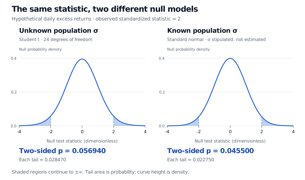
Here Ft24 is the cumulative distribution function of that null statistic. Approximately 5.69% of repeated samples from this zero-mean normal model would produce an absolute t statistic of at least 2. Each tail contributes about 2.85%. This is an area under a distribution, not the height of the density curve at 2.
Two null densities with tails shaded beyond minus 2 and plus 2. Student t with 24 degrees of freedom gives two-sided p 0.056940; standard normal gives 0.045500. Each distribution is labelled, with dimensionless statistic on the horizontal axes and null probability density on the vertical scale.
Original hypothetical comparison. The left panel uses estimated population volatility; the right assumes population volatility is known. Shading continues beyond the displayed range to infinity in both directions.
If the population standard deviation were known to be 0.003, the appropriate standardized statistic would instead be normal under this model. Its numerical value would still be 2, but the two-sided p-value would be
Read the result without turning it into a verdict on the strategy
At a predeclared 5% significance level, the t result does not reject zero mean: 0.056940>0.05. This does not establish that the mean is zero. The same data would reject at a predeclared 10% level; moving the threshold after seeing the result does not preserve the original decision rule.
A value just above 0.05 and one just below it need not represent materially different evidence. Report the value and the design, rather than assigning the strategy a pass/fail badge. The American Statistical Association's statement summary emphasizes interpretation in context, transparent reporting and the limits of threshold-based decisions.
Three tempting translations are wrong:
“There is a 5.69% probability that the null is true.” The calculation assumes the null while generating its reference distribution. A posterior probability for the null requires a Bayesian model with prior probabilities and alternatives.
“There is a 94.31% probability the strategy works or replicates.” Neither 1−p nor p supplies that forecast. Replication depends on the true effect, future sample design, selection and stability.
“The effect is small because the p-value is large.” A p-value mixes the observed departure with its sampling uncertainty. It does not measure economic magnitude.
The estimated mean here is 12 basis points per day, irrespective of the p-value. A matching 95% confidence interval is approximately −0.38 to 24.38 basis points per day. It includes zero, consistent with the two-sided 5% test, and shows considerable uncertainty about magnitude. This range describes a procedure with repeated-sampling coverage under the model; it is not a 95% posterior probability statement.
For trading, ask separately whether the return definition includes fees, spread, impact, financing and borrow. Evidence against exactly zero gross return does not demonstrate positive net value, acceptable risk or sufficient capacity.
The tail depends on the research question
If the study had specified an upper one-sided alternative H1:μ>0 in advance, the observed positive statistic would give
p+=PH0(T≥2)≈0.028470.
That is a different question and rejection rule. Halving a two-sided result after discovering the estimated sign is a form of selection. Specify direction, statistic, sampling window, stopping rule and significance level before inspecting the data. Other tests can define two-sided extremeness differently, particularly with discrete outcomes; “double a tail” is not a universal recipe.
A small p-value can be produced by a large search
For this continuous t test under its null, the p-value is uniformly distributed between 0 and 1 before observing the sample. More generally, a valid p-value satisfies
PH0(P≤α)≤α.
Here P denotes the random p-value across repeated samples. The statement controls false rejection under the null; it does not say what fraction of reported discoveries are false.
Now imagine 20 independent tests whose nulls are all true, each evaluated at 5%. The chance of at least one false rejection is
1−(1−0.05)20≈0.6415.
That 64.15% illustrates why selecting the smallest p-value among many backtests is a different procedure from running one prespecified test. Correlated strategies change this particular calculation, while the search problem remains. Disclose variants and use an appropriate multiple-testing procedure or a genuinely untouched validation design. Repeatedly checking a fixed-sample test and stopping at the first attractive result also requires a procedure designed for sequential monitoring.
Finally, all of these numerical probabilities rely on the reference model. Serial dependence, heavy tails and changing return distributions can undermine a naive small-sample t calculation. Choosing a more suitable variance estimator or resampling design requires assumptions too. A precise p-value cannot repair a poorly specified experiment.
For the sample-versus-population distinction and standard-error calculation, Basic Statistics and Regression is available in full with a free signed-in account. For the derivation connecting normal samples, t inference and test–interval duality, read Confidence Intervals and Hypothesis Testing; the full lesson requires membership, with a public preview.
Sources
John A. Rice, Mathematical Statistics and Data Analysis, 3rd edition, §9.2.1, “Specification of the Significance Level and the Concept of a p-value” — interpretation and specifying the level before analysis.
George Casella and Roger L. Berger, Statistical Inference, 2nd edition, §8.3.4, Definition 8.3.26, Theorem 8.3.27 and Example 8.3.28 — validity under the null and the two-sided normal-sample t calculation.