Understand hypothesis tests through a return-sample t-test, rejection rules, error rates, power and the distinction between statistical evidence and a tradable edge.
Hypothesis test
A hypothesis test is a rule for deciding whether sample data provide enough evidence to reject a specified claim about a population or data-generating process. The claim is the null hypothesis, H0; the competing claim is the alternative, H1. The rule is designed to control how often it rejects a true null under stated assumptions.
For a quant, the question might be whether a strategy's expected return differs from zero, whether a regression coefficient vanishes, or whether observed losses fit a risk model. A positive backtest average is an observation. A test asks how unusual the corresponding statistic would be under the null model. Neither the observation nor the test by itself establishes a durable trading edge.
Specify the question before seeing the answer
A useful test starts with the population, sampling model, hypotheses, statistic and decision threshold. Suppose the quantity of interest is the mean daily excess return μ of one fixed strategy, using returns measured consistently against a specified cash benchmark. A two-sided question is
H0:μ=0,H1:μ=0.
It looks for departures in either direction. A predeclared positive-edge question instead uses H0:μ≤0 against H1:μ>0. The choice changes the rejection region. Choosing the positive direction only after observing a positive average does not preserve the original error guarantee.
The significance levelα is a chosen upper bound on the probability of rejecting a true null. More generally, if the null permits several parameter values, that bound must hold across all of them. A 5% level is a design convention, not a law of economics. Fix the sample window, return definition, direction and analysis protocol before using the result to make a confirmatory claim. Rice's treatment explicitly places the level choice before the data analysis; it also distinguishes the null tail probability from a posterior probability.
A short return history near the decision boundary
Consider an original hypothetical sample of 25 daily excess returns. For this calculation, stipulate independent, identically distributed normal returns with unknown mean and unknown population standard deviation. This is a teaching model, not a claim that real strategy returns satisfy it.
The observed summaries are:
Quantity
Decimal-return units
Basis points
Sample mean, xˉ
0.0012
12 per day
Sample standard deviation, s
0.0030
30 for daily returns
Estimated standard error, s/25
0.0006
6 for the daily mean
One basis point is 0.0001 in decimal-return units. The standard deviation describes variation across daily returns; the standard error describes the sampling uncertainty of the estimated mean. Here s uses divisor n−1, not n:
s2=n−11i=1∑n(xi−xˉ)2.
Under H0:μ=μ0 and the stated normal model, the random statistic
T=S/nXˉ−μ0∼tn−1.
Estimating the population standard deviation is why the exact reference distribution is Student's t. For the observed sample and μ0=0,
tobs=0.003/250.0012=2,n−1=24.
Write t24,0.975 for the 97.5th percentile of that distribution. At a two-sided 5% level, reject when
∣tobs∣>t24,0.975≈2.0639.
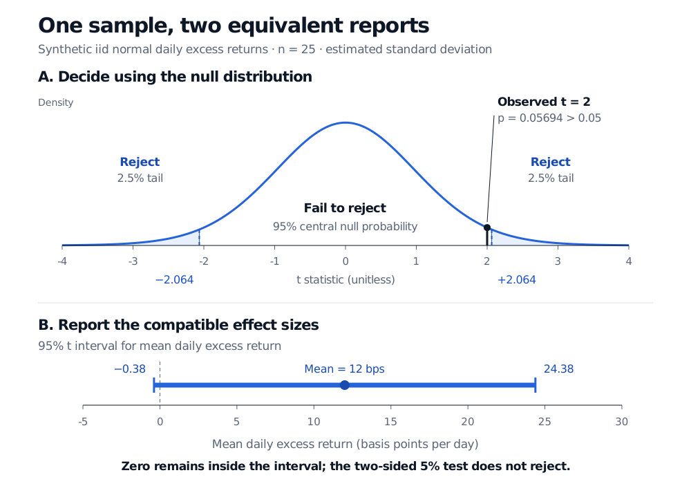
The observed value 2 is inside the non-rejection region. Equivalently, its two-sided p-value is
p=PH0(∣T∣≥2)≈0.05694>0.05.
We fail to reject the zero-mean null at the predeclared 5% level. This does not establish that the true mean is zero, and it does not turn a positive sample average into a negative finding about profitability. The NIST one-sample mean guide sets out the different reference statistics for estimated and known population standard deviations.
Synthetic iid normal return example: observed t equals 2, inside the two-sided 5% non-rejection region bounded by minus and plus 2.064. The matching 95% interval for mean daily excess return is minus 0.38 to plus 24.38 basis points, containing zero.
Original calculation for the stipulated normal model, with 24 degrees of freedom. Shaded rejection tails have total null probability 5%; the interval uses the same sample and assumptions.
That is roughly −0.38 to +24.38 basis points per day. Zero lies inside it, agreeing with the test. This duality applies to the matching two-sided test and interval under the same model and variance estimate. The interval also reveals how imprecisely the mean is estimated. Its 95% refers to the procedure's repeated-sampling coverage, not a 95% posterior probability assigned to this fixed mean. NIST's interval guide explains that distinction.
Why substituting a normal cutoff changes the conclusion
If the population standard deviation were genuinely known to equal 0.003, the statistic would instead be Z=(Xˉ−μ0)/(σ/n), standard normal under the null. Its observed value would still be 2, but the two-sided p-value would be about 0.04550, below 5%. The numerical statistic alone does not determine the decision; its reference distribution matters.
In this sample, 0.003 is an estimate, so the known-volatility calculation answers a different problem. Treating an estimated volatility as known can overstate precision. Likewise, a right-tailed t-test predeclared for positive mean would give about 0.02847 here; switching tails after seeing the sample is a change of procedure.
Two errors, and the power to detect an effect
Decision
Null true
Specified alternative true
Reject H0
Type I error
Detection
Fail to reject H0
No false rejection
Type II error
A Type I error is a false rejection. A Type II error misses a real departure from the null. Power is the probability of rejection at a specified alternative; it is one minus the Type II error probability there. Power depends on effect size, noise, sample size and the test rule. There is no single power number without specifying an alternative and any relevant nuisance parameters.
At a fixed sample size, tightening the rejection rule lowers the false-alarm rate but can also make real effects harder to detect. A short sample may fail to reject both when the null is true and when a modest edge exists. If the business question is whether the mean is negligibly small, an appropriately designed equivalence test with a predeclared tolerance addresses that question; ordinary non-rejection does not.
A research decision needs more than the test
The model assumptions do the work. Serial dependence can invalidate s/n as the standard error, and non-normal observations remove this small-sample exact t reference. A central limit theorem may support an approximation in a suitable larger-sample setting, but the variance estimate and dependence assumptions still need justification. Volatility clustering, outliers and changing regimes merit investigation rather than a mechanical switch to a familiar cutoff.
Statistical significance also leaves the economic question open. Define whether returns are before or after transaction costs, funding and borrow charges; assess size and uncertainty against the return required to deploy capital. A very small effect can become statistically detectable in a large sample while remaining uneconomic. The American Statistical Association's principles emphasize that significance does not measure effect magnitude or practical importance.
Finally, the search is part of the experiment. If 20 independent tests each have exact size 5% and every null is true, the probability of at least one rejection is
1−(1−0.05)20≈0.6415.
That is about 64.15%, even though each individual test is valid. The independence assumption is essential to this particular formula; correlated strategy trials need a different calculation. Repeatedly inspecting the same accumulating sample or selecting the best variant also changes the procedure. Report the search, use suitable multiple-testing controls or a prespecified sequential design, and keep a genuinely untouched evaluation sample where appropriate. A p-value from the winning backtest does not automatically account for all the trials that produced it.
For the underlying sample summaries, Basic Statistics and Regression is available in full with a free signed-in account; its public page is a preview. Confidence Intervals and Hypothesis Testing develops the normal-family pivot, test and interval together; its public page is a preview and the full lesson requires membership.
Sources
John A. Rice, Mathematical Statistics and Data Analysis, 3rd edition, §§9.2–9.2.1 (testing, error rates and p-values) and §9.3 (test–interval duality). Numerical scenario and figure are original.