Why repeated independent observations stabilise an average: weak and strong laws, an exact trading example, a Chebyshev bound, and the limits of convergence.
Law of large numbers
The law of large numbers says that the average of many observations approaches their expected value, under suitable assumptions. In its standard independent and identically distributed form, it explains why a sample average can estimate a population mean. It also explains why averaging simulated payoffs can estimate a model value.
The word average matters. A profitable strategy's average profit per trade may stabilise while its cumulative profit keeps fluctuating, its next trade remains risky, and a small account runs out of cash. The theorem concerns a specified probability model; collecting more observations does not establish that the model describes the market.
A trading edge is a mean, not a schedule
Suppose a hypothetical trade produces a net profit of USD 6 with probability 55%, or a net loss of USD 4 with probability 45%. Assume fixed position size and that these outcomes repeat independently, with the same probabilities each time. These are stipulated model probabilities, not estimates from a backtest.
The law says this average approaches USD 1.50 per trade. It does not require any individual trade to earn USD 1.50; that outcome is impossible here. Nor must the average improve with each additional trade. It can move away from its target before returning closer.
Independence makes the variance of the sum add across trades. Therefore
E[Xˉn]=1.50,Var(Xˉn)=n24.75.
Its standard error, meaning the standard deviation across repeated samples of the same size, is 24.75/n USD per trade:
Number of trades
Standard error of average, USD per trade
25
0.9950
100
0.4975
400
0.2487
Quadrupling the number of independent trades halves this uncertainty scale. It does not promise to halve the error in whichever sample you happen to observe.
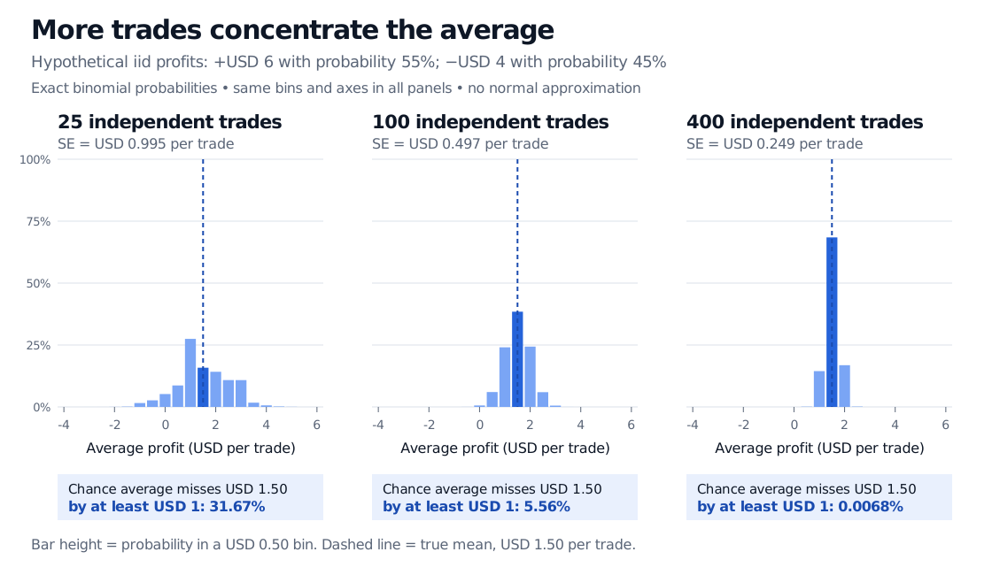
Exact sample-mean distributions for 25, 100 and 400 hypothetical independent trades concentrate near USD 1.50. Standard errors are USD 0.995, 0.497 and 0.249 per trade. Exact probabilities of an error at least USD 1 are 31.67%, 5.56% and 0.0068%, respectively.
Original hypothetical model. All panels use the same USD 0.50 bins and probability axes. Bars group exact binomial probabilities over the full support; the tail figures use the ungrouped distribution, including equality at the USD 1 threshold. No normal approximation is used.
To see where those probabilities come from, let Kn count winning trades. Then Kn has a binomial distribution, and
Xˉn=n6Kn−4(n−Kn)=10nKn−4.
At n=100, an average error of at least USD 1 occurs when K100≤45 or K100≥65. Adding those exact binomial probabilities gives about 5.56%. This finite-sample calculation uses the entire specified distribution. The law of large numbers alone does not supply that number.
Two meanings of “approaches”
Let X1,X2,… be independent and identically distributed, abbreviated iid, with
E[∣X1∣]<∞,μ=E[X1].
The finite absolute mean ensures the expected value is a finite, well-defined number, without cancellation between infinite positive and negative contributions.
The weak law states that for every fixed tolerance ε>0,
P(∣Xˉn−μ∣≥ε)⟶0.
This is convergence in probability: choose a large sample size, and an average outside any fixed tolerance becomes increasingly unlikely.
The strong law states
P(n→∞limXˉn=μ)=1.
This is almost-sure convergence: along almost every infinite sequence of outcomes, the running average eventually stays within each fixed positive tolerance. The point at which it stays there depends on the realised sequence and the tolerance. There is no promised universal trade count after which all possible samples behave well.
Almost-sure convergence implies convergence in probability; the converse fails for general sequences of random variables. Under the iid, finite-absolute-mean assumptions just stated, both laws hold. The distinction concerns the strength of their conclusions, not two competing forecasts. MIT's strong-law notes develop the pathwise result.
A short proof, and what it assumes
With the extra condition σ2<∞, Chebyshev's inequality gives a direct proof of the weak law:
P(∣Xˉn−μ∣≥ε)≤ε2Var(Xˉn)=nε2σ2⟶0.
Berkeley's probability notes present this variance-based argument. Finite variance is needed for this proof and its bound. It is not necessary for the iid law of large numbers itself; finite absolute mean suffices. An infinite-variance distribution may obey the law while lacking the familiar standard-error formula.
For our USD 1 tolerance and 100 trades, Chebyshev gives
P(∣Xˉ100−1.5∣≥1)≤10024.75=0.2475.
The bound is 24.75%, compared with the model's exact 5.56%. That looseness is the price of using only a mean and variance. To make this bound at most 5%, n≥495 is sufficient. It is not the smallest sample size that the specified binomial model might require.
The central limit theorem answers a further question: under its assumptions, what is the approximate distribution of the scaled errorn(Xˉn−μ)/σ? The LLN establishes concentration; a normal approximation requires additional reasoning. Neither theorem turns a single trade's two-point distribution into a normal distribution.
The account still has to survive
Let cumulative profit be Sn=∑i=1nXi. Its expected value is 1.5n USD, but its standard deviation is 24.75n USD. At 100 and 400 trades, that standard deviation is about USD 49.75 and USD 99.50. Average uncertainty shrinks while absolute uncertainty in cumulative dollars grows.
Now give the trader USD 12 of capital, no borrowing or external funding, and require stopping if capital reaches zero. Three initial losses exhaust that capital. Their probability is
0.453=0.091125=9.1125%.
That is just one possible failure event, not the account's total ruin probability. The positive model mean does not remove it. An infinite sequence of potential trade outcomes can obey the LLN even though a finite account cannot keep trading along every path. Reinvesting a fraction of wealth also introduces compounding; a dollar-profit average is not a geometric growth rate.
A losing streak does not make a win due. In this iid model, the next win probability remains 55% after any observed history. Long-run balance emerges through averaging, without a compensating force that remembers past losses.
When more data answers the wrong question
For dependent observations with finite second moments,
The covariance terms may prevent the iid uncertainty calculation from applying. In the extreme, repeat the same random profit every time: Xi=Y for all i. Then Xˉn=Y forever; more rows have added no independent information. Some dependent processes do satisfy laws of large numbers, but require suitable additional conditions.
A regime change raises another problem. An average combining old and new strategy behaviour need not estimate the current regime's mean. A longer backtest can make a historical mixture look precise while leaving today's edge uncertain. Likewise, a Monte Carlo estimate can converge accurately to the expectation of a misspecified model.
For the underlying moment calculations, the Mathematics Primer lesson is available in full with a free signed-in account. For a longer treatment connecting convergence, sample-size bounds and normal approximations, read Laws of Large Numbers and the Central Limit Theorem; the full lesson requires membership.
Sources
Dimitri P. Bertsekas and John N. Tsitsiklis, Introduction to Probability, 2nd edition (2008), §5.2, pp.269–272, and §5.5, pp.280–282 — sample means, the Chebyshev proof and the distinction between weak and strong convergence. The trading example and figure are original.