A random walk accumulates independent shocks. Calculate exact inventory probabilities, separate steps from levels, and see how scaled walks lead to Brownian motion.
Random walk
A random walk is a sequence formed by adding successive independent, identically distributed random increments to a starting value. It is a basic model for how uncertainty accumulates through time: each new shock changes the current position, and earlier shocks remain embedded in later positions.
For a quant, the distinction between a shock and an accumulated position matters. Order flow might generate a toy random walk in a dealer's inventory; a price model might instead put a random walk in log-price. Those choices have different units and economic implications. Calling something a random walk does not establish that markets actually have independent increments, or that a trading strategy has an edge.
The step is independent; the level remembers
With a fixed starting position S0=a, write
Sn=a+i=1∑nXi.
The increments Xi are independent and identically distributed, often abbreviated iid. The simple random walk uses only two possible increments:
P(Xi=1)=p,P(Xi=−1)=1−p.
It is symmetric when p=1/2 and biased otherwise. More general random walks can have normally distributed increments, jumps of many sizes or vector-valued steps. The word random alone does not specify their distribution.
The positions S1,S2,… are not independent. Both S4 and S5 contain the first four shocks. If each increment has finite mean m and variancev, independence gives
E[Sn]=a+nm,Var(Sn)=nv.
For deterministic a and j≤k, the shared shocks also give Cov(Sj,Sk)=jv. Independent changes can therefore produce strongly dependent levels. Treating a sequence of accumulated positions as independent observations can make statistical evidence look stronger than it is.
For the simple walk, m=2p−1 and v=4p(1−p). Its standard deviation is 2np(1−p): doubling the number of steps doubles the variance, but multiplies the standard deviation by 2. At p=0 or p=1, the motion is deterministic and that uncertainty vanishes.
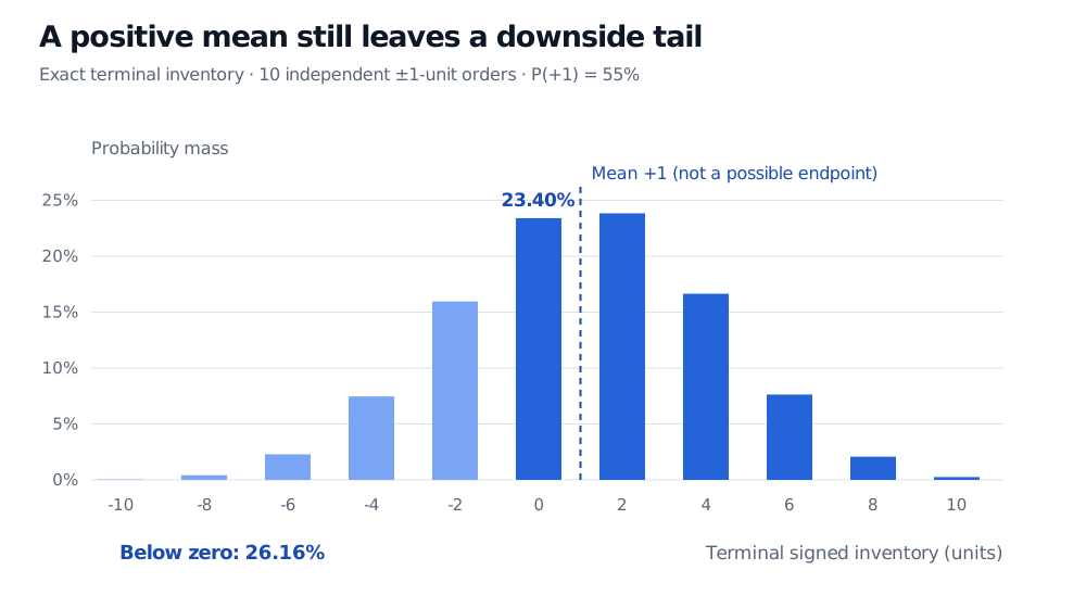
Consider a deliberately simplified dealer who starts with zero inventory. Each incoming order changes inventory by one unit: a dealer purchase adds +1 and a dealer sale adds −1. Assume orders are independent, with the same 55% purchase probability each time. There are no inventory limits, hedges or changes in quoting policy in this hypothetical model. Inventory is a signed number of units, not a stock price or a profit.
The standard deviation is approximately 3.146 units, substantially larger than the expected change. A positive mean does not make a negative endpoint unlikely enough to ignore.
Count the purchases. If U is that count, then U has a binomial distribution with ten trials and success probability 0.55. The remaining 10−U orders are sales, so S10=2U−10. In general, for a simple walk starting at zero,
P(Sn=2u−n)=(un)pu(1−p)n−u,u=0,1,…,n.
Returning to zero at order ten means five purchases and five sales:
P(S10=0)=(510)(0.55)5(0.45)5≈23.4033%.
A negative endpoint requires at most four purchases:
P(S10<0)=u=0∑4(u10)(0.55)u(0.45)10−u≈26.1563%.
Exact distribution of terminal inventory after ten independent plus-or-minus-one-unit orders with purchase probability 55%. Negative inventory has probability 26.16%, zero has probability 23.40%, and the mean is plus one unit, which is not an attainable endpoint.
Original hypothetical inventory model; bars show exact probabilities, not a simulated histogram. The dashed mean is between the attainable endpoints zero and two.
There is a useful lattice check: after ten unit steps, only even positions are possible. The expected value is +1, but no realised endpoint can equal +1. An expected value is a probability-weighted average, not necessarily a possible outcome. After an odd number of these steps, returning exactly to zero is impossible.
The endpoint does not describe the exposure on the way
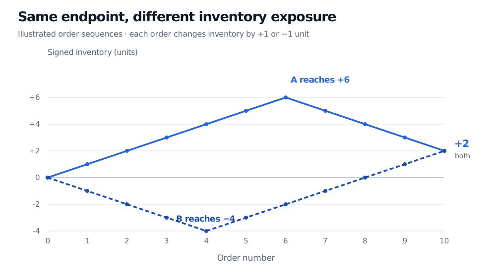
Six purchases followed by four sales leave inventory at +2, after first reaching +6. Four sales followed by six purchases also end at +2, after first reaching −4. Under the stipulated iid model, these particular ordered paths have the same probability: each contains six purchases and four sales.
Two illustrated ten-order paths both end at plus two inventory units. Path A buys six times then sells four times and reaches plus six; path B sells four times then buys six times and reaches minus four.
Illustrated sequences, not market data. Equal terminal inventory does not imply equal interim exposure. Straight connectors guide the eye between discrete order events.
A desk with a four-unit absolute inventory limit could follow the second sequence but would breach its limit on the first. Once a rule stops, hedges or changes the process at a boundary, the unconstrained terminal binomial formula no longer describes the resulting controlled inventory. Likewise, the probability of being at zero at a specified time differs from the probability of ever returning to zero or hitting a risk limit. Those are path questions.
For an indefinitely continued, one-dimensional symmetric unit-step walk, return to the starting point occurs with probability one. That statement supplies neither a finite deadline nor a bound on the distance travelled before return. It should not be used to justify holding a losing position until it recovers. Shreve's 1997 CMU notes, Chapter 8, introduce the related first-passage problem.
From lattice steps to Brownian motion
A random walk is also a bridge from discrete models to Brownian motion. For iid increments with mean m and finite, strictly positive variance v, the central limit theorem describes a single standardised endpoint:
nvSn−a−nmdN(0,1).
For a path limit on [0,1], put the centred walk on grid times k/n and rescale its vertical movement:
Z(n)(k/n)=nvSk−a−km,k=0,…,n.
Join these grid values by linear interpolation. Donsker's invariance principle states that these random continuous functions converge in distribution to standard Brownian motion, in the uniform topology. It concerns distributions of entire paths; it does not say that any chosen sequence of simulated pictures must settle onto one Brownian trajectory. Khoshnevisan's notes define the interpolation and state the theorem precisely.
The scaling is essential. Running an unscaled unit-step walk faster makes its variance grow without bound. For a symmetric walk with physical time step Δt, increments ±σΔt instead accumulate variance σ2T over T/Δt steps. This motivates diffusion models; it does not prove that real price shocks satisfy their assumptions.
What a random-walk assumption leaves unresolved
A symmetric walk with integrable increments is a martingale: its conditional expected next position equals its current position. A biased walk has a predictable mean change; subtracting nm produces a martingale under the stipulated iid law. This is a statement about the model and its information set. Market efficiency does not follow from drawing a noisy path, and an efficient-market argument need not require zero expected returns or constant volatility.
An arithmetic walk used directly for a stock price can eventually produce negative prices. Modelling log-price avoids that particular problem, but exponential conversion changes price expectations: zero expected log-increment does not imply zero expected price return. Geometric Brownian motion makes that distinction in continuous time.
Finally, iid increments exclude changing shock distributions and dependence between successive shocks. A dealer's inventory policy, clustered volatility, jumps or changing market conditions can defeat the simple specification. The useful workflow is to state what is walking, its units, the step law and the horizon, then ask whether the application needs an endpoint probability, a path probability or a different model.
For the discrete foundations, Simple Random Walks — Symmetric and Asymmetric develops step moments, the Markov property and recurrence. The full lesson requires membership; its public page provides a preview.
Practice: a fair walk can still lose
A toy strategy has eight independent trades. Each earns USD 2 or loses USD 2, each with probability 1/2. It starts at zero cumulative profit, and there are no costs or early stopping. Find its expected cumulative profit, standard deviation and probability of ending at USD −8 or below.
Answer. Each trade has mean zero and variance 4 USD2. Eight independent trades therefore give mean USD 0, variance 32 USD2, and standard deviation 32≈USD 5.657. If U is the number of profitable trades, cumulative profit is 2U−2(8−U)=4U−16 dollars. A result at or below −8 requires U≤2, so
The zero mean balances gains against losses across possible outcomes. It does not prevent a loss on an individual path.
Sources
Grimmett and Stirzaker, Probability and Random Processes, 3rd edition, §3.9: simple random walks, iid increments and their structural properties. Local grounding text read.
Steven Shreve, Stochastic Calculus and Finance, CMU lecture notes dated 25 July 1997, with Prasad Chalasani and Somesh Jha, Chapter 8 and §13.4: first passage and linearly interpolated scaled walks. This is the 1997 notes text, not the later Volume I textbook.