Stochastic calculus turns noisy price changes into trading gains and a corrected chain rule. Build the Itô integral from holdings, squared increments and a reproducible Brownian-grid example.
Stochastic calculus
Stochastic calculus is the mathematics of integrating and transforming random processes whose paths can be too rough for ordinary calculus. In finance it gives a precise meaning to the gains from changing a position through time, and explains why an option's curvature contributes to its change in value.
The essential adjustment is easy to state: for Brownian motion, squared price-driver increments accumulate instead of disappearing. The resulting calculus keeps a second-order term that the ordinary chain rule drops. This article develops the continuous Brownian case; processes with jumps require additional terms.
Decide the holding, then observe the move
Suppose a stock price is St. At each trading time ti, choose a holding Hti shares and keep it through the next interval. The stock-trading gain is
GN=i=0∑N−1Hti(Sti+1−Sti).
Each term has units shares × currency per share = currency. It uses the holding chosen before the price change, rather than selecting the position after seeing whether that change was profitable. A holding depending on tomorrow's return would describe a different, anticipative strategy.
The information available by time t is denoted Ft. An adapted process uses information available at that time. The general trading-integral formulation uses predictable holdings: positions determined from information available before the increment they earn. Left-point step holdings chosen from Fti give the basic construction; continuous adapted holdings also fit the predictable framework.
A stochastic integral extends this gains sum to continuous time. For standard Brownian motion W, a predictable integrand H satisfying
E[∫0THt2dt]<∞
has a square-integrable Itô integral∫0THtdWt, constructed by approximating H with simple holdings in mean square. For a continuous adapted H with suitable integrability, shrinking left-point sums provide that approximation. It is not an ordinary integral of Ht times a derivative Wt′: Brownian paths are almost surely nowhere differentiable.
A useful check is the Itô isometry:
E(∫0THtdWt)2=E[∫0THt2dt].
Under the stated condition this integral has mean zero and is a martingale as its upper limit varies. These claims concern integration against the Brownian driver under the probability measure being used. They do not say that every actual trading strategy has zero expected profit. A stock generally has a drift and a financing leg too. Kogan's MIT notes introduce the integral through this non-anticipating, left-point construction.
One identity exposes the difference
Take Ht=Wt, with W0=0, and abbreviate ΔWi=Wti+1−Wti. Ordinary algebra gives
Wti+12−Wti2=2WtiΔWi+(ΔWi)2.
Summing telescopes the left side. Consequently, on every finite grid, exactly,
i=0∑N−1WtiΔWi=21(WT2−i=0∑N−1(ΔWi)2).
No probability theorem has been used yet. The correction is the realised sum of squared increments, not automatically T.
For Brownian motion on deterministic partitions whose largest interval tends to zero, that squared-increment sum converges to T in mean square. This is quadratic variation, written [W]T=T. Passing to the limit gives
∫0TWtdWt=21(WT2−T).
The expectation check catches the common mistake. Since E[WT2]=T, the Itô result has mean zero. The ordinary-chain-rule answer WT2/2 would have mean T/2.
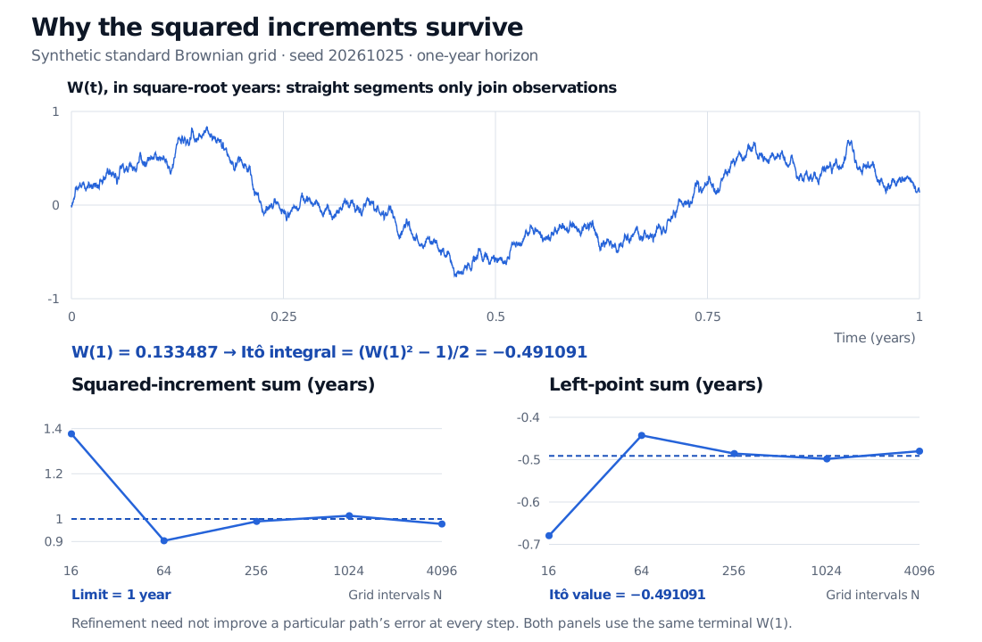
Here is a reproducible synthetic example, using time in years, T=1, seed 20261025 and 4096 independent Gaussian increments with variance 1/4096. The sampled path finishes at W1=0.133487 (rounded). Its final diagnostics are:
Quantity
Value, in years
Finite squared-increment sum
0.977736
Finite left-point sum
−0.479959
Itô integral implied by the terminal value, (W12−1)/2
−0.491091
The Brownian driver has units year, so both products have units years; these diagnostics are not currency P&L. The finite sum obeys the exact algebraic identity. Its difference from the limiting integral is half of one minus the squared-increment sum. Refining this particular path need not reduce the error at every step.
A synthetic one-year Brownian grid ends at W1=0.133487. Nested quadratic sums fluctuate around 1 year. Left-point sums fluctuate around the Itô value −0.491091 years, with final 4096-step sum −0.479959 years.
Original synthetic Brownian-grid illustration, not a market price. Coarse grids use the same sampled path. Straight segments only join displayed observations; the finite grid does not prove a continuous-path theorem.
The convention matters. For this integrand, the symmetric endpoint sum ∑i(Wti+Wti+1)ΔWi/2 equals WT2/2 exactly on a finite grid. Its limit defines the corresponding Stratonovich integral. That convention supports an ordinary-looking chain rule, but the symmetric weight is not the start-of-interval holding in the trading ledger. Converting between the two calculi requires the quadratic-variation correction; simply changing the integral symbol changes the meaning.
The chain rule keeps curvature
An Itô stochastic differential equation
dXt=atdt+btdWt
means the integral equation Xt=X0+∫0tasds+∫0tbsdWs. Under the usual integrability conditions, and for a function f(t,x) once continuously differentiable in time and twice in space, Itô's lemma gives
df(t,Xt)=(ft+atfx+21bt2fxx)dt+btfxdWt.
The derivatives are evaluated at (t,Xt). The extra bt2fxx/2 term measures curvature interacting with accumulated squared noise. For a linear function it vanishes; for a convex function it is nonnegative. Writing (dWt)2=dt is convenient shorthand for quadratic variation, not an equality between an individual squared Gaussian increment and its time step.
For example, geometric Brownian motion satisfies dSt=μStdt+σStdWt. Applying the rule to logSt gives
dlogSt=(μ−21σ2)dt+σdWt.
Dropping curvature would overstate the log drift. It would also give an incorrect exponential simulation formula.
From a gains integral to an option price
Consider a frictionless market with a non-dividend-paying stock and a cash account earning a constant continuously compounded rate r. A self-financing portfolio with wealth Vt and Δt shares obeys
dVt=ΔtdSt+r(Vt−ΔtSt)dt.
Rebalancing transfers money between stock and cash; it does not inject new wealth. If a smooth option value is v(t,St), Itô's rule supplies its curvature contribution 21σ2St2vSSdt. Matching the diffusion with delta hedging, Δt=vS, and matching the self-financing drift yields the Black–Scholes equation
vt+21σ2S2vSS+rSvS−rv=0.
Thus the gamma term comes from the same squared increments seen in the finite-grid identity. This argument assumes continuous trading, the stated diffusion model, financing and sufficient regularity. Discrete hedging, costs and jumps change the realised hedge result.
Keep two probability descriptions separate. Under the physical measureP, the stock drift μ describes its modelled real-world expected return. Under a risk-neutral measure Q, this non-dividend-paying model uses drift r and a Brownian motion WQ. With the necessary integrability, discounted self-financing wealth is a Q-martingale. This pricing representation does not assert that investors expect only the risk-free return in the real world.
1. On four observation intervals spanning one year, a sampled Brownian-driver path has increments 1/2,−1/4,3/4,−1/2, in year. Starting from zero, compute the left-point sum ∑WtiΔWi. Can you replace its squared-increment sum by one year exactly?
Answer. The successive starting levels are 0,1/2,1/4,1, and the terminal level is 1/2. Direct multiplication gives
0+21(−41)+4143+1(−21)=−167=−0.4375 years.
Independently, the squared-increment sum is 1/4+1/16+9/16+1/4=9/8 years, and the identity gives ((1/2)2−9/8)/2=−7/16 years. Substituting T=1 instead would give −3/8=−0.375 years: the limiting-integral value implied by the endpoint, not this finite gains sum.
2. Let dXt=0.3dt+0.4dWt, with time in years and X in arbitrary value units. At Xt=2, what drift and diffusion coefficients does Xt2 have?
Answer. Itô's formula gives d(Xt2)=(0.6Xt+0.16)dt+0.8XtdWt. At Xt=2, the drift coefficient is 1.36 value-units squared per year, and the diffusion coefficient is 1.6 value-units squared per square-root year. Ordinary calculus would miss the 0.16 drift contribution from the squared diffusion coefficient.
Sources
Steven E. Shreve, Stochastic Calculus and Finance, Carnegie Mellon lecture notes prepared by Prasad Chalasani and Somesh Jha, July 25, 1997, §§14.6, 14.8–14.9 and 15.1: holdings-based construction, square-integrable integral, Brownian self-integral and the chain rule. The local file is not the later textbook volume with a similar name.
John C. Hull, Options, Futures, and Other Derivatives, 9th Global Edition, §§14.2 and 14.6, plus the Chapter 14 appendix: Brownian increment scaling and the second-order change-of-variables formula.