Delta hedging offsets an option position’s local stock sensitivity. Follow a funded two-year hedge, audit every rebalance, and see why neutrality does not remove all risk.
Delta hedging
Delta hedging means trading the underlying to offset a position’s current sensitivity to small changes in its price. A writer of a call option has negative stock sensitivity; buying shares offsets it. As the option’s delta changes, the share holding must be adjusted.
The hedge controls a particular exposure. It also creates purchases, sales, interest and possible borrowing. A useful hedge calculation therefore answers two questions together: how many shares should I hold, and how does the cash account pay for them?
The sign comes from the position
Let V(t,S) be the price of a long option per underlying share, and let n be the signed number of contracts, each covering m shares. Positive n means long; negative means short. If the stock holding is h shares, its combined delta is
Δposition=nm∂S∂V+h.
The delta-neutral target is h=−nmΔ. A short call with positive long-option delta therefore needs a positive stock holding. A long call needs a short stock holding. The multiplier matters: contract count alone is not a share count.
A delta-neutral portfolio has zero first-order sensitivity at the current inputs. For a small spot change, holding time and volatility fixed, the linear terms approximately cancel. The OIC’s delta guide describes delta as a theoretical local estimate and explains why it changes. It does not make a large spot move linear.
Follow the financing through two years
Consider an original, hypothetical contract written on 24 October 2026: one European call on one share, strike USD 100, expiring 24 October 2028. This is a one-share unit for teaching, rather than a standard 100-share listed contract.
Use a binomial option pricing model with two one-year steps. The stock begins at 100; in each year it multiplies by either u=1.2 or d=0.8. Cash earns, or borrowing costs, 5% annual effective each year, so the annual accumulation factor is R=1.05. There are no dividends. Fractional shares and unrestricted borrowing are allowed; fees, bid–ask spreads, credit losses and interim collateral calls are excluded.
This is a stipulated finite-state model, not a fitted market forecast. Its risk-neutral probability is
q=u−dR−d=1.2−0.81.05−0.8=85.
That pricing weight follows from replication, not a claim that the stock has a 62.5% real-world chance of rising.
At expiry the stock is 144, 96 or 64, and the call pays 44, 0 or 0. Rolling these payoffs backward gives the year-one call values
Cu=1.05(5/8)44+(3/8)0=26.190476,Cd=0,
and the opening value
C0=1.05(5/8)Cu+(3/8)Cd=15.589569.
Displayed decimals are rounded; the hedge calculations retain exact fractions.
The opening premium helps buy the hedge
At any node, the finite-state hedge ratio matches the difference between the next two option values:
h=Sup−SdownCup−Cdown.
It is an exact replication ratio for those two successor states. It need not equal a smooth model’s derivative at every possible stock price.
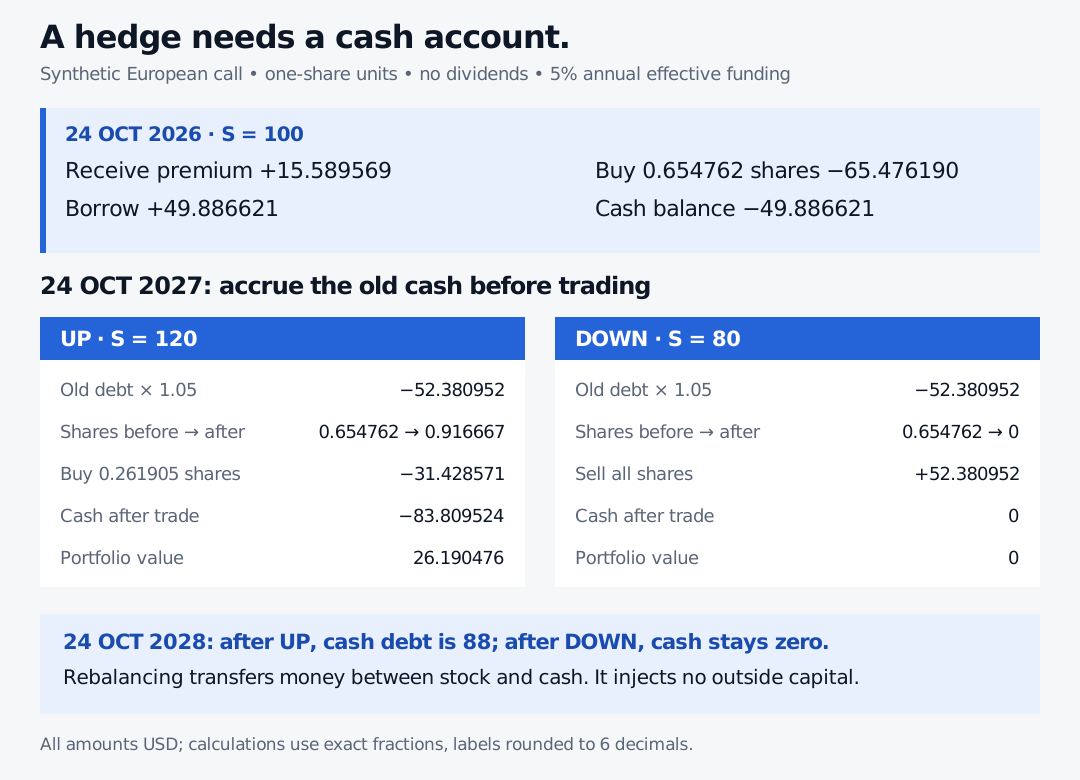
Here B is cash in dollars, positive for a deposit and negative for debt. Buying the shares costs 65.476190. The writer receives the call premium of 15.589569 and borrows the remaining 49.886621. The stock-plus-cash portfolio has value C0, matching the short-call liability; the combined position begins at net value zero.
The premium is received once. It is neither free trading profit nor a payment repeated each time shares are bought.
At year one, accrue interest before resizing
Before the next trade, the old cash balance has become
B0R=−52.380952….
If the stock rises to 120, the old shares plus accrued debt are worth 26.190476, exactly the call value at that node. The next year can end at 144 or 96, so the new holding is
hu=144−9644−0=1211.
Buy only the additional 11/12−55/84=11/42 shares. They cost (11/42)120=31.428571…. Financing that purchase through the same account gives
Bu=−52.380952…−31.428571…=−83.809524….
The rebalance changes the allocation between shares and debt, not the portfolio’s value.
If the stock falls to 80, the call is worth zero: neither of its next-year states produces a positive payoff. Sell all 55/84 shares for 52.380952 and repay the accrued debt. Both the stock holding and the cash balance become zero.
A dated stock-and-cash ledger with an opening premium-funded hedge and separate UP and DOWN rebalances.
Original synthetic USD ledger, one-share European call, two annual steps, no dividends, 5% annual effective funding, fractional shares and unrestricted borrowing; no costs or collateral calls. Values rounded; calculations use exact fractions.
Settle every path, including both ways to 96
After the UP rebalance, the debt grows to exactly 88 at expiry. After DOWN there is no remaining holding or debt.
Two-year path
Terminal stock
Stock held at expiry
Terminal cash
Hedge wealth
Call liability
Writer’s net
UP → UP
144
132
−88
44
−44
0
UP → DOWN
96
88
−88
0
0
0
DOWN → UP
96
0
0
0
0
0
DOWN → DOWN
64
0
0
0
0
0
All monetary columns are USD per one-share call. “Stock held” here means its terminal dollar value. The two routes to 96 use different trading histories, yet both settle correctly. This is dynamic replication inside the stated model. It does not produce a profit from selling at the replication price.
Self-financing is a ledger rule
Write hi and Bi for shares and cash just after a rebalance at ti. For a no-dividend asset, with accumulation factor Ri until the next trading date, wealth just before trading is
Xi+1−=hiSi+1+BiRi.
To change the holding to hi+1, update cash by
Bi+1=BiRi−(hi+1−hi)Si+1.
These equations define the frictionless self-financing portfolio: share purchases are financed by existing cash or additional borrowing, while sales replenish cash. No external money is injected at the rebalance. Self-financing does not mean debt-free, cost-free or immune to losses.
With trading cost ki+1≥0, subtract it from the cash update too. Wealth then falls by that cost at execution. Dividends, different borrowing and lending rates, stock-borrow charges and margin transfers need their own dated entries. A collateral demand can exhaust usable cash even when a pricing model reports a good hedge.
For the underlying finite-state construction, read The Binomial Model, available as a full public sample. The derivation there uses continuous-rate discounting; the example here deliberately uses annual effective funding.
What breaks when the stock leaves the tree?
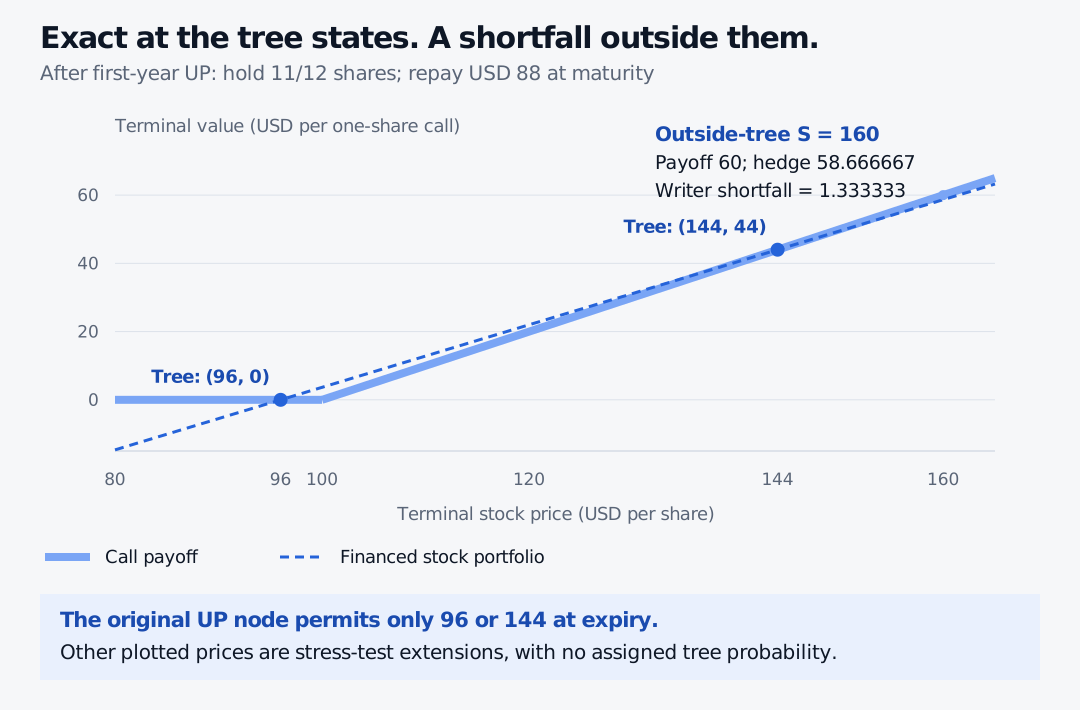
After the first UP move, keep the prescribed 11/12 shares and terminal debt of 88. Now suppose the terminal stock is 160. That is an out-of-model stress, not a fifth path admitted by the original tree.
The hedge is worth (11/12)160−88=58.666667, while the call pays 60. Defining hedging error as hedge wealth minus payoff gives
εT=58.666666…−60=−34.
The writer is short USD 1.333333 per call unit. The two-state hedge matched the liabilities at 96 and 144; it did not match every possible terminal stock price.
After first-year UP, the financed stock line matches the call at permitted tree prices 96 and 144 but falls short at an explicitly outside-tree price 160.
Original synthetic terminal comparison after first-year UP. Only 96 and 144 are permitted successor prices. The line elsewhere is a stress-test extension, not a probability scenario admitted by the original tree.
A live hedge keeps moving
In the ideal Black–Scholes model, continuously adjusting the derivative delta and financing the stock position replicates a European claim under the model’s assumptions. A real hedge trades at discrete times, at executable prices, using uncertain inputs.
Several effects survive a stock hedge:
Gamma changes the delta as spot moves. A short vanilla call is short gamma: after an upward move, its writer generally needs more stock; after a downward move, less. Larger moves between trades can create substantial error.
Vega measures sensitivity to volatility marks. Stock has no direct option vega, so offsetting delta does not remove a volatility repricing.
Theta and funding continue while the hedge is held. Time decay received by a short option is not pure profit; it must be assessed alongside convexity losses, financing and other changes.
Jumps and execution constraints can move the stock before a rebalance is possible. Spreads, impact, trading halts and funding limits make the actual hedge differ from the ideal target. American early exercise also changes the timing of obligations.
More frequent hedging can reduce diffusion-driven discretisation error when the model is appropriate. It also increases turnover and may increase costs; improvement is not guaranteed on every realised path. Calendar schedules and delta bands are choices about risk and execution cost, not a universal “best” frequency. CME’s explanation of dynamic hedge ratios reinforces the need to resize as delta changes.
1. Resize the hedge. A writer is short 10 call contracts, each covering 100 shares. Long-call delta rises from 0.55 to 0.62; stock is USD 103 at the rebalance. The existing holding was neutral at the old delta. Ignoring costs, what trade restores neutrality, and what happens to cash?
Answer. The target rises from 10×100×0.55=550 shares to 10×100×0.62=620. Buy 70 shares, costing USD 7,210. Cash after accruing the old balance falls by 7,210; if funded by borrowing, debt rises by that amount. Buying 620 more shares would confuse the new total with the required trade. The option premium is not paid or received again.
2. Test “neutral means safe.” One short call on one share is locally delta-neutral with stock. Long-call gamma is 0.03 per dollar. Over a USD 4 spot rise, hold time and volatility fixed, keep the stock hedge unchanged, and use only the second-order Taylor term. What residual mark-to-market change do you estimate, before costs?
Answer. The linear terms cancel; the short option retains gamma −0.03. Its estimated residual is −21(0.03)(4)2=−0.24, a USD 0.24 loss. This is a local frozen-time approximation, not a full trading-period profit calculation: actual time passage, funding, volatility changes and higher-order terms also matter.
Sources
Hull, John C., Options, Futures, and Other Derivatives, 9th Global Edition, Chapter 13 and §§19.4, 19.7–19.8. Local text checked for finite-state replication, dynamic share hedging, funding, gamma/theta and vega. The worked tree and practice questions above are original.
Shreve, Steven E., Stochastic Calculus and Finance, CMU lecture notes prepared by Prasad Chalasani and Somesh Jha, 25 July 1997, §§3.3.1–3.3.2 and 3.4. Local text checked for predictable holdings, the self-financing wealth recurrence and replication; this is the dated lecture-note file, rather than the later Volume I textbook.
CME Group: Options Delta — The Greeks — contract hedge ratios and dynamic rebalancing. Futures hedge units differ from the stock-share ledger used here.